CS 664 Lecture 19 Layers RANSAC panoramas epipolar

CS 664 Lecture #19: Layers, RANSAC, panoramas, epipolar geometry Some material taken from: • David Lowe, UBC • Jiri Matas, CMP Prague http: //cmp. felk. cvut. cz/~matas/papers/presentations/matas_beyond-ransac_cvprac 05. ppt

Announcements § Paper report due on 11/15 § Please choose a final project soon – Email me a proposal after you get your paper report graded – Which will be soon after 11/15! § Project must have a research component – Talk to me if you have questions § Next quiz Thursday 11/3 – coverage through last lecture § PS#2 due November 8 2

Handling large motions § None of these optical-flow based techniques work well for large motions or for really textured scenes – Need “just right” amount of texture! § A standard solution for larger motions is to do this “coarse to fine” – Run on a low resolution version of the image – Apply this as a warp, then increase resolution – These methods have some ugly properties • But a number of people think they work 3

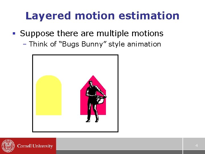
Layered motion estimation § Suppose there are multiple motions – Think of “Bugs Bunny” style animation 4

Layered motion algorithms § Global affine fit with IRLS should give us the dominant motion – Assuming it’s >50% of the image – Outlier pixels (low IRLS weights) are doing something else, so we can focus on them § Need to find what the motions are, which pixels belong to each region – If we know one, we could compute the other – Classical application of EM – To initialize, compute local affine fits and cluster in 6 -dimensional space 5

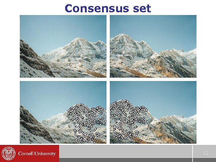
RANSAC § Extremely popular way to do model fitting in the presence of noisy data – One of the best algorithms in the vision toolkit § Algorithm: – Select a random sample of data points – Find model that best fits these points(LS) – Find all other data points that like this model • Consensus set § Parameters: number of iterations, sample size, consensus set “tolerance” 6

Example: registration 7

Example: multiple motions 8

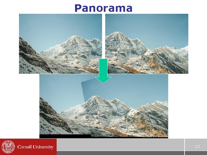
RANSAC for sparse registration § Given an interest-point operator – Corner detector, or SIFT (we will cover this) § Assume we’re looking at a plane – Planar homography • Homography = projective transformation • Planar homography = 2 D affine homography – Application: recognizing panoramas • Brown & Lowe, ICCV 2003 http: //www. cs. ubc. ca/~mbrown/panorama 9

Recognizing panoramas 10

Feature extraction (SIFT) 11

Consensus set 12

Panorama 13

Completing the panorama § We have a lot of pairwise panoramas – How do we create a complete panorama? – A connected set should be a panorama § How to create the image? – Pairwise registrations aren’t globally consistent § Camera parameters come in two classes – Intrinsic: focal length, pixel size & spacing – External: rigid body motion (6 d. o. f. ) – For a given panorama, we will assume the parameters are only rotation & focal length 14

Bundle adjustment § We have a set of cameras with their parameters old, and need to add a new image and estimate its parameters – Find the that makes the feature points line up as closely as possible • Minimize the “reprojection error” • Robustify this, to handle outliers – Actually, we minimize both old and § Non-linear least squares problem – Usually solved with Levenberg-Marquadt 15

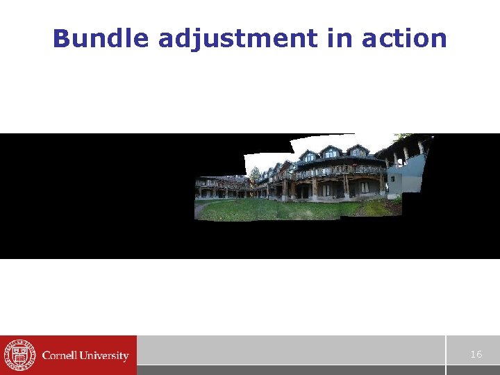
Bundle adjustment in action 16

Results 17

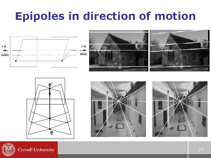
Epipolar geometry § Where could a point in I 1 appear in I 2? – Motion: anywhere nearby – Stereo: anywhere horizontally nearby • Why just horizontal? – Assume a stationary scene 18

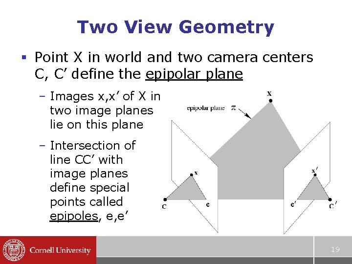
Two View Geometry § Point X in world and two camera centers C, C’ define the epipolar plane – Images x, x’ of X in two image planes lie on this plane – Intersection of line CC’ with image planes define special points called epipoles, e, e’ e e 19

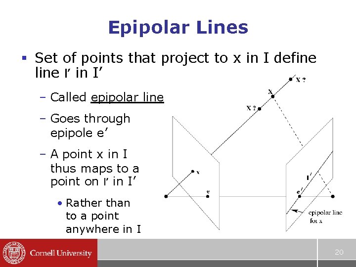
Epipolar Lines § Set of points that project to x in I define l’ in I’ – Called epipolar line – Goes through epipole e’ – A point x in I thus maps to a point on l’ in I’ • Rather than to a point anywhere in I 20

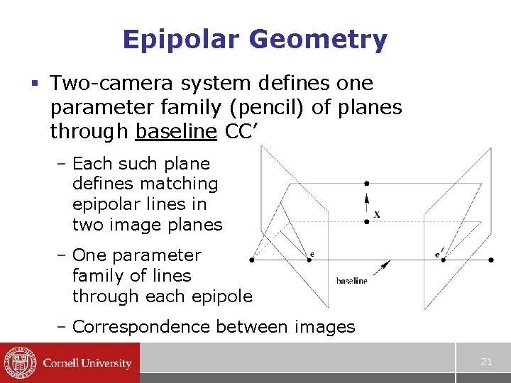
Epipolar Geometry § Two-camera system defines one parameter family (pencil) of planes through baseline CC’ – Each such plane defines matching epipolar lines in two image planes – One parameter family of lines through each epipole – Correspondence between images 21

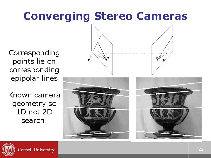
Converging Stereo Cameras Corresponding points lie on corresponding epipolar lines Known camera geometry so 1 D not 2 D search! 22

Epipoles in direction of motion e’ e 23