CS 6501 Deep Learning for Computer Graphics Basics

CS 6501: Deep Learning for Computer Graphics Basics of Neural Networks, and Training Neural Nets I Connelly Barnes

Overview • Simple neural networks • Perceptron • Feedforward neural networks • Multilayer perceptron and properties • Autoencoders • How to train neural networks • Gradient descent • Stochastic gradient descent • Automatic differentiation • Backpropagation

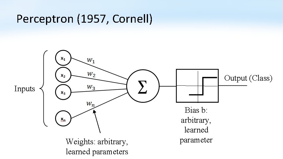
Perceptron (1957, Cornell) Output (Class) Inputs Weights: arbitrary, learned parameters Bias b: arbitrary, learned parameter

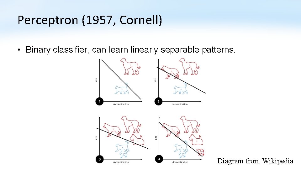
Perceptron (1957, Cornell) • Binary classifier, can learn linearly separable patterns. Diagram from Wikipedia

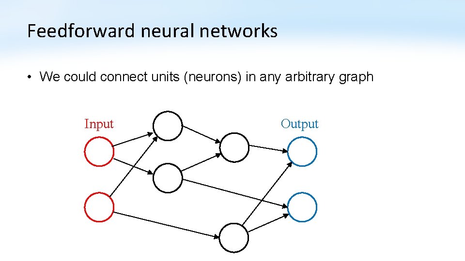
Feedforward neural networks • We could connect units (neurons) in any arbitrary graph Input Output

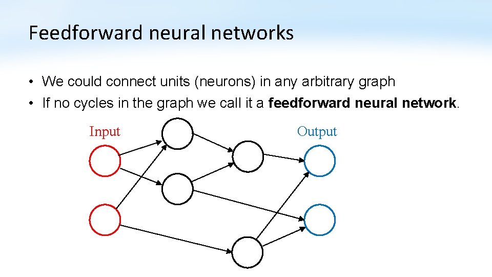
Feedforward neural networks • We could connect units (neurons) in any arbitrary graph • If no cycles in the graph we call it a feedforward neural network. Input Output

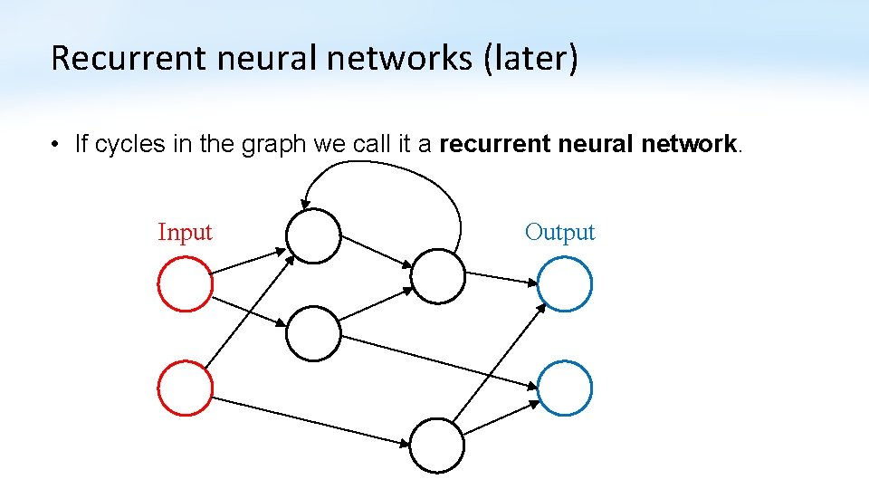
Recurrent neural networks (later) • If cycles in the graph we call it a recurrent neural network. Input Output

Overview • Simple neural networks • Perceptron • Feedforward neural networks • Multilayer perceptron and properties • Autoencoders • How to train neural networks • Gradient descent • Stochastic gradient descent • Automatic differentiation • Backpropagation

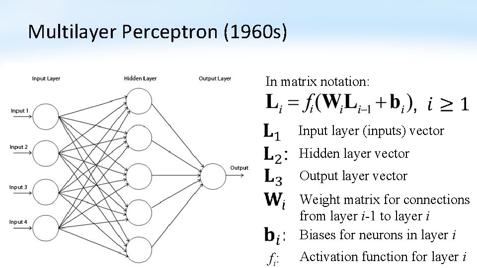
Multilayer Perceptron (1960 s) In matrix notation: i Input layer (inputs) vector Hidden layer vector Output layer vector Weight matrix for connections from layer i-1 to layer i Biases for neurons in layer i f i: Activation function for layer i

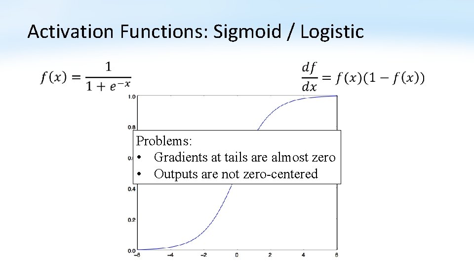
Activation Functions: Sigmoid / Logistic Problems: • Gradients at tails are almost zero • Outputs are not zero-centered

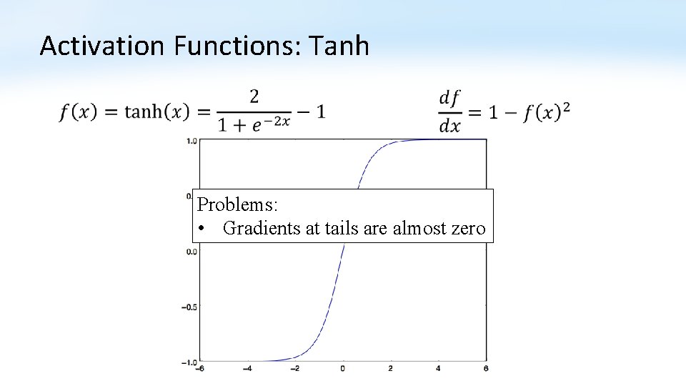
Activation Functions: Tanh Problems: • Gradients at tails are almost zero

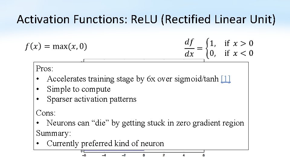
Activation Functions: Re. LU (Rectified Linear Unit) Pros: • Accelerates training stage by 6 x over sigmoid/tanh [1] • Simple to compute • Sparser activation patterns Cons: • Neurons can “die” by getting stuck in zero gradient region Summary: • Currently preferred kind of neuron

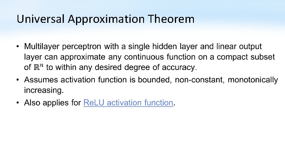
Universal Approximation Theorem •

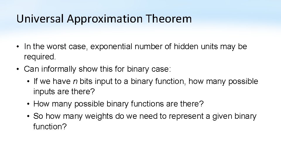
Universal Approximation Theorem • In the worst case, exponential number of hidden units may be required. • Can informally show this for binary case: • If we have n bits input to a binary function, how many possible inputs are there? • How many possible binary functions are there? • So how many weights do we need to represent a given binary function?

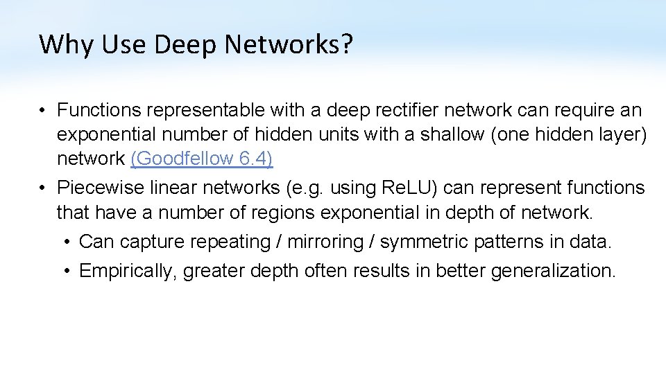
Why Use Deep Networks? • Functions representable with a deep rectifier network can require an exponential number of hidden units with a shallow (one hidden layer) network (Goodfellow 6. 4) • Piecewise linear networks (e. g. using Re. LU) can represent functions that have a number of regions exponential in depth of network. • Can capture repeating / mirroring / symmetric patterns in data. • Empirically, greater depth often results in better generalization.

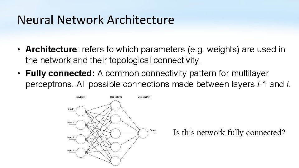
Neural Network Architecture • Architecture: refers to which parameters (e. g. weights) are used in the network and their topological connectivity. • Fully connected: A common connectivity pattern for multilayer perceptrons. All possible connections made between layers i-1 and i. Is this network fully connected?

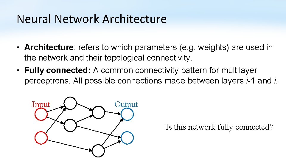
Neural Network Architecture • Architecture: refers to which parameters (e. g. weights) are used in the network and their topological connectivity. • Fully connected: A common connectivity pattern for multilayer perceptrons. All possible connections made between layers i-1 and i. Input Output Is this network fully connected?

How to Choose Network Architecture? • Long discussion • Summary: • Rules of thumb do not work. • “Need 10 x [or 30 x] more training data than weights. ” • Not true if very low noise • Might need even more training data if high noise • Try many networks with different numbers of units and layers • Check generalization using validation dataset or cross-validation.

Overview • Simple neural networks • Perceptron • Feedforward neural networks • Multilayer perceptron and properties • Autoencoders • How to train neural networks • Gradient descent • Stochastic gradient descent • Automatic differentiation • Backpropagation

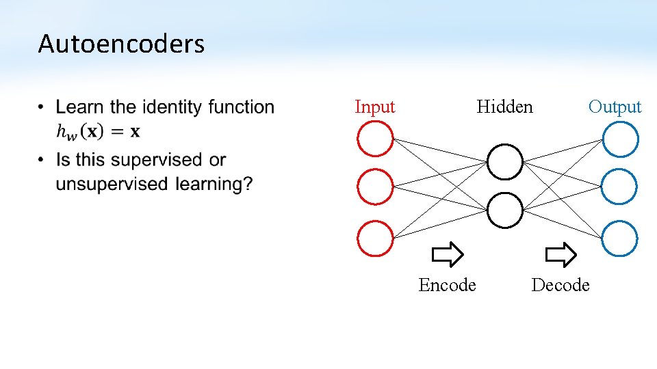
Autoencoders • Input Hidden Encode Output Decode

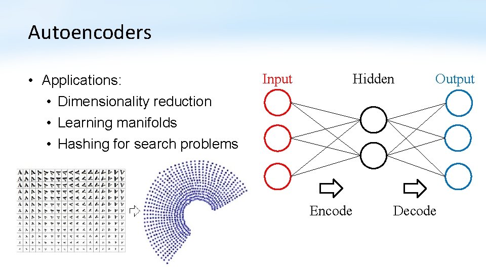
Autoencoders • Applications: • Dimensionality reduction • Learning manifolds • Hashing for search problems Input Hidden Encode Output Decode

Overview • Simple neural networks • Perceptron • Feedforward neural networks • Multilayer perceptron and properties • Autoencoders • How to train neural networks • Gradient descent • Stochastic gradient descent • Automatic differentiation • Backpropagation

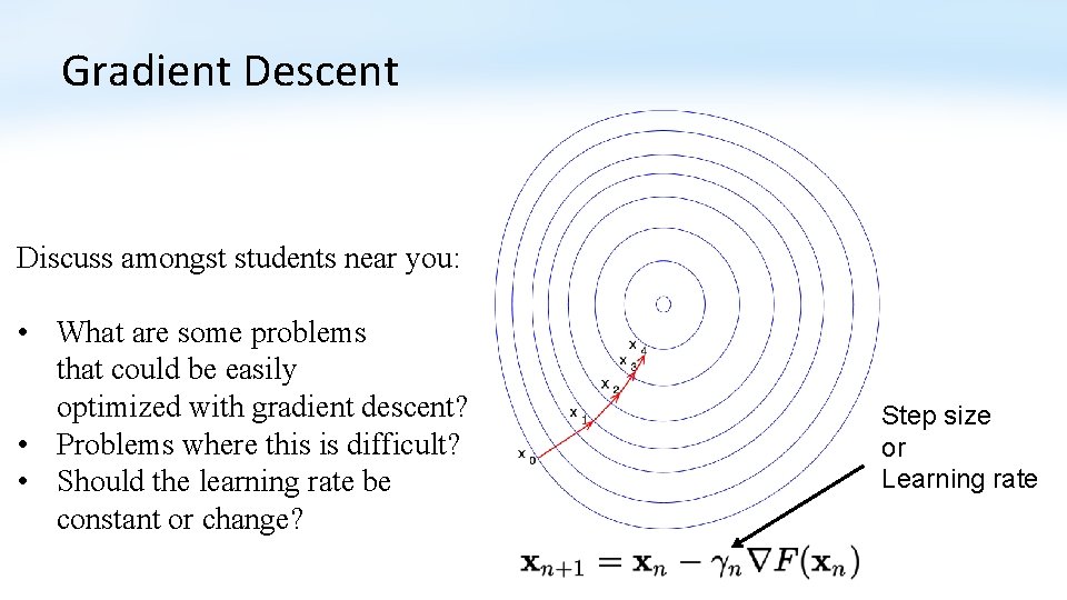
Gradient Descent Discuss amongst students near you: • What are some problems that could be easily optimized with gradient descent? • Problems where this is difficult? • Should the learning rate be constant or change? Step size or Learning rate

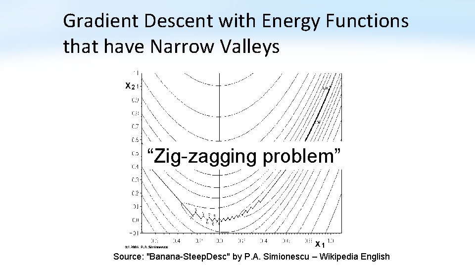
Gradient Descent with Energy Functions that have Narrow Valleys “Zig-zagging problem” Source: "Banana-Steep. Desc" by P. A. Simionescu – Wikipedia English

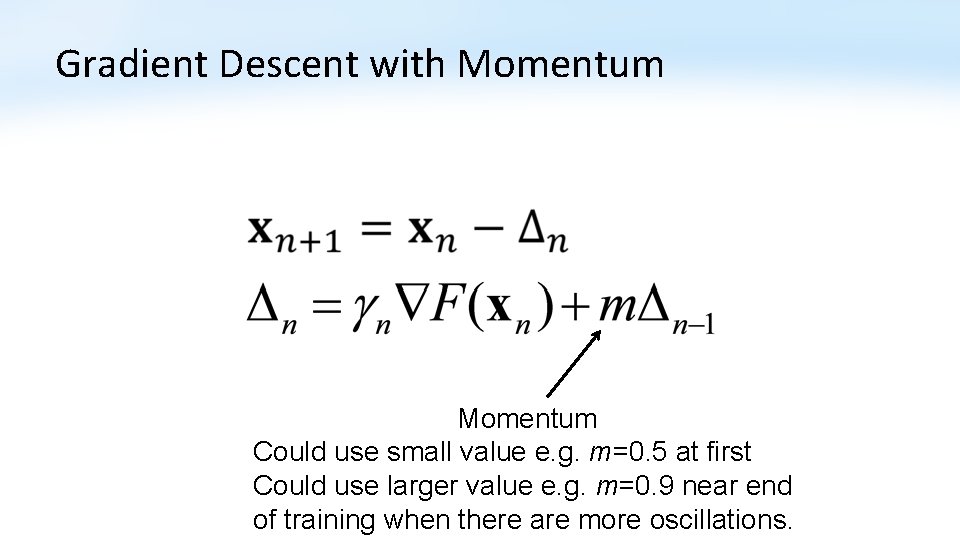
Gradient Descent with Momentum Could use small value e. g. m=0. 5 at first Could use larger value e. g. m=0. 9 near end of training when there are more oscillations.

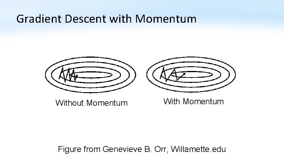
Gradient Descent with Momentum Without Momentum With Momentum Figure from Genevieve B. Orr, Willamette. edu

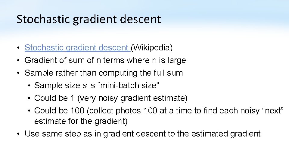
Stochastic gradient descent • Stochastic gradient descent (Wikipedia) • Gradient of sum of n terms where n is large • Sample rather than computing the full sum • Sample size s is “mini-batch size” • Could be 1 (very noisy gradient estimate) • Could be 100 (collect photos 100 at a time to find each noisy “next” estimate for the gradient) • Use same step as in gradient descent to the estimated gradient

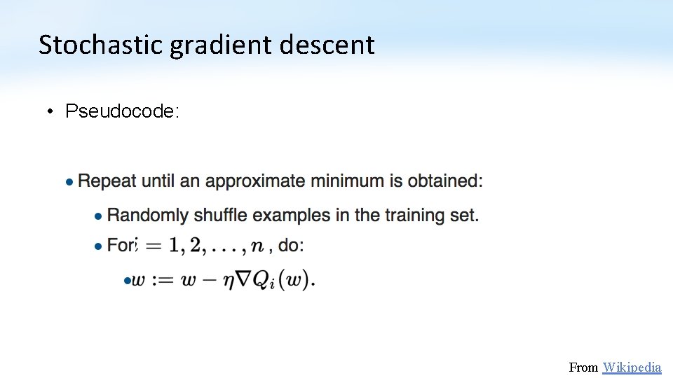
Stochastic gradient descent • Pseudocode: From Wikipedia

Problem Statement • Take the gradient of an arbitrary program or model (e. g. a neural network) with respect to the parameters in the model (e. g. weights). • If we can do this, we can use gradient descent!

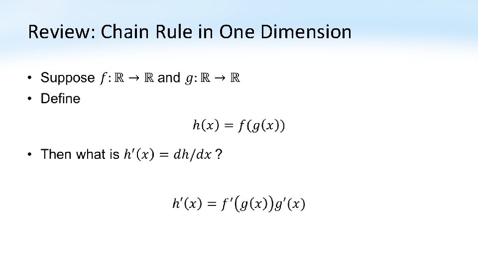
Review: Chain Rule in One Dimension •

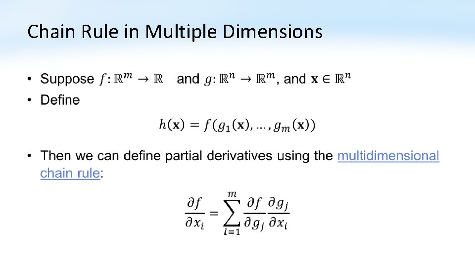
Chain Rule in Multiple Dimensions •

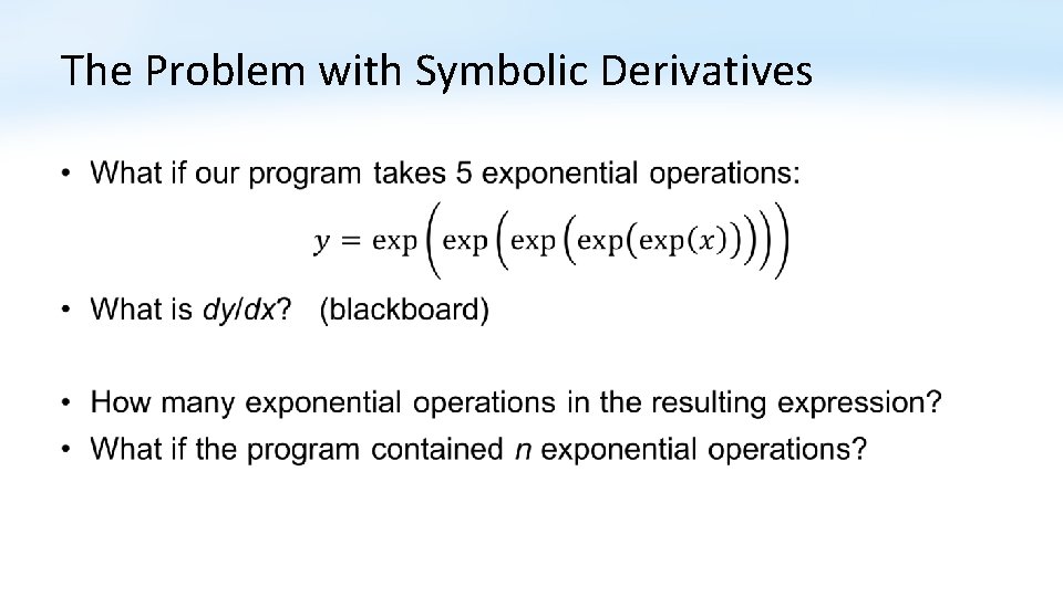
The Problem with Symbolic Derivatives •

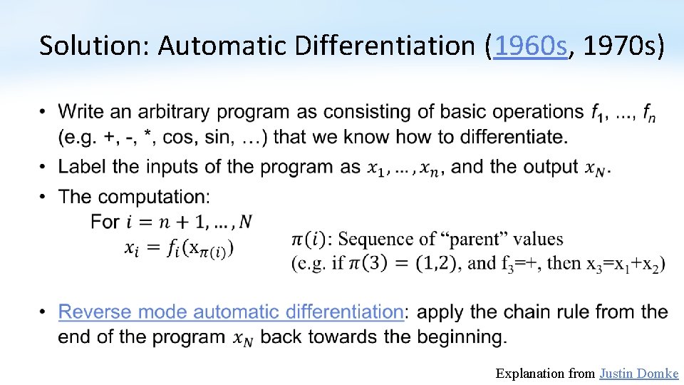
Solution: Automatic Differentiation (1960 s, 1970 s) • Explanation from Justin Domke

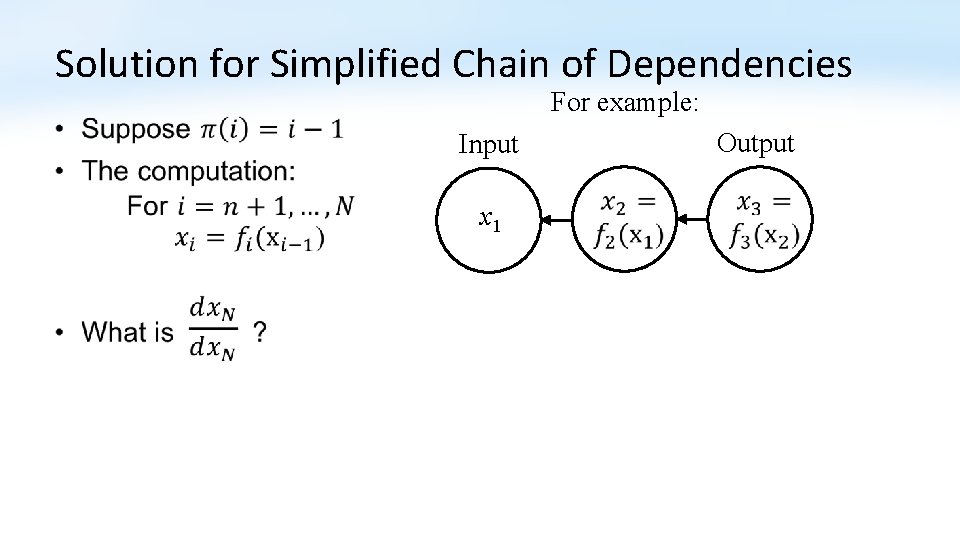
Solution for Simplified Chain of Dependencies For example: • Output Input x 1

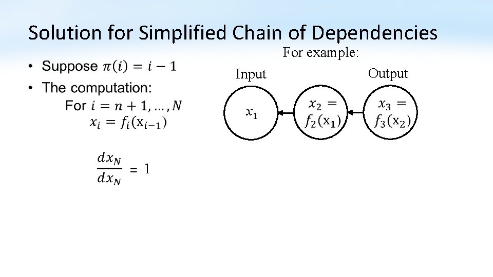
Solution for Simplified Chain of Dependencies For example: • Output Input x 1 1

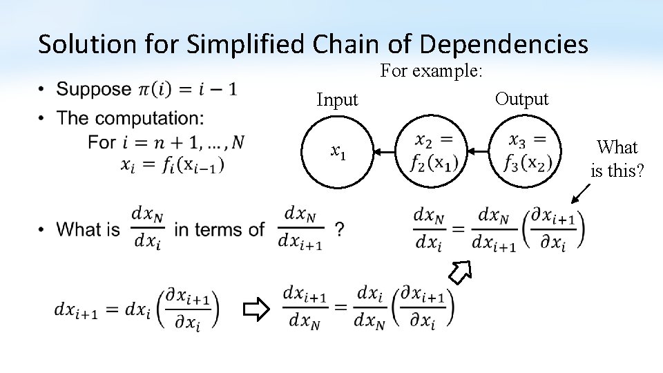
Solution for Simplified Chain of Dependencies For example: • x 1 Output Input What is this?

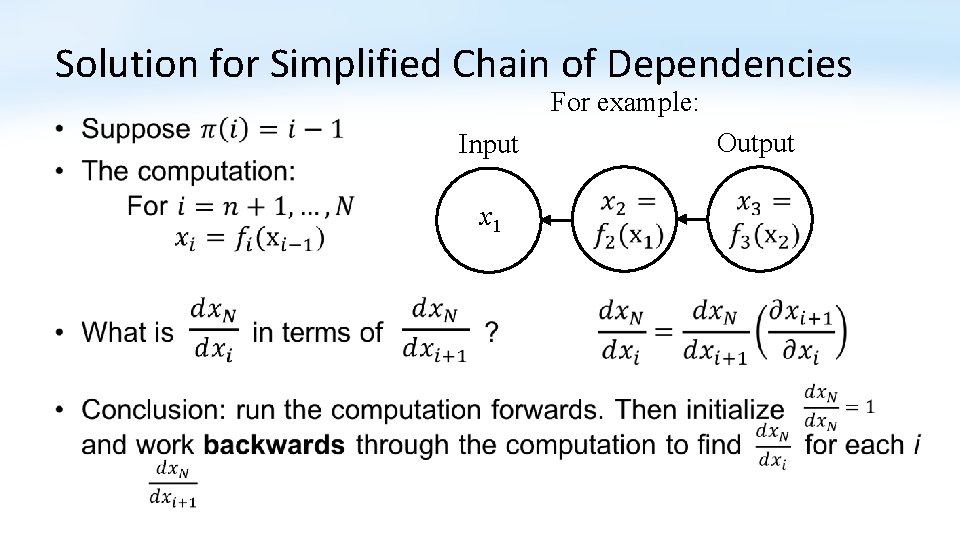
Solution for Simplified Chain of Dependencies For example: • Output Input x 1

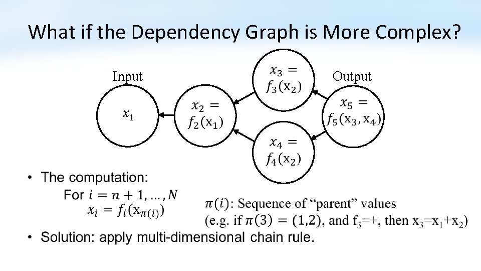
What if the Dependency Graph is More Complex? Input x 1 Output

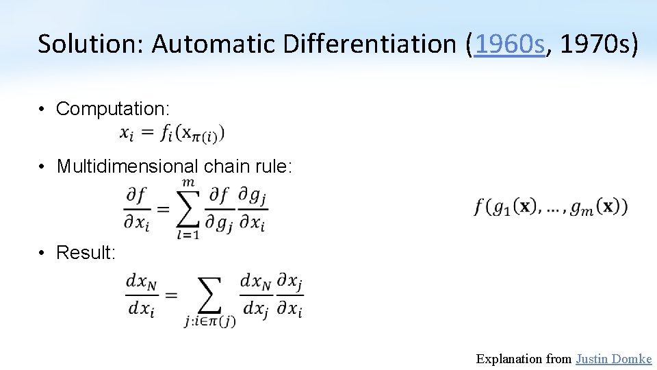
Solution: Automatic Differentiation (1960 s, 1970 s) • Computation: • Multidimensional chain rule: • Result: Explanation from Justin Domke

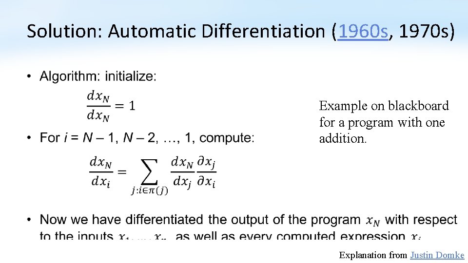
Solution: Automatic Differentiation (1960 s, 1970 s) • Example on blackboard for a program with one addition. Explanation from Justin Domke

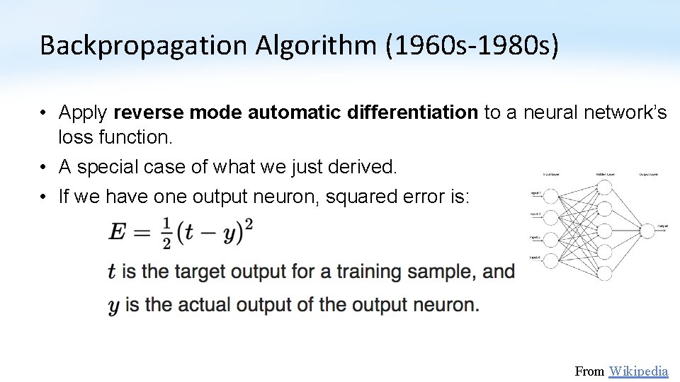
Backpropagation Algorithm (1960 s-1980 s) • Apply reverse mode automatic differentiation to a neural network’s loss function. • A special case of what we just derived. • If we have one output neuron, squared error is: From Wikipedia

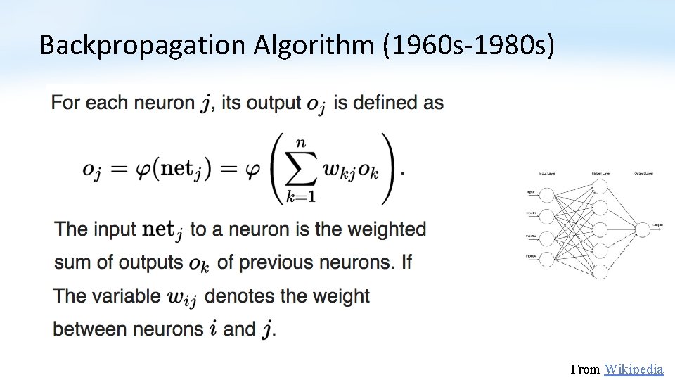
Backpropagation Algorithm (1960 s-1980 s) From Wikipedia

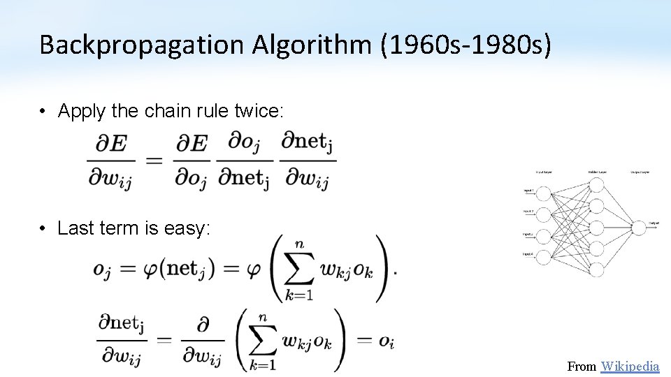
Backpropagation Algorithm (1960 s-1980 s) • Apply the chain rule twice: • Last term is easy: From Wikipedia

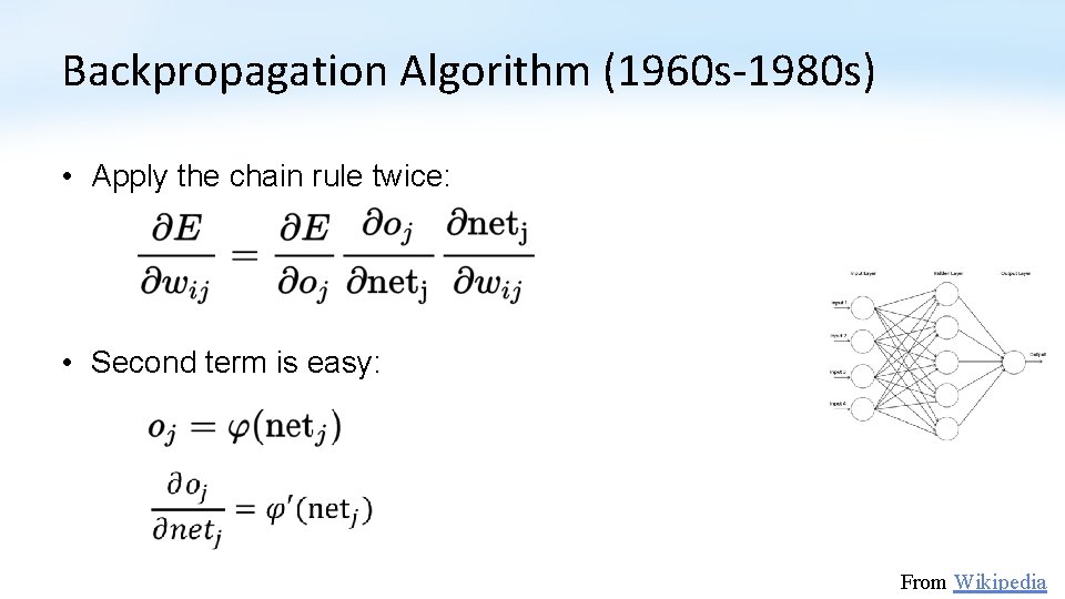
Backpropagation Algorithm (1960 s-1980 s) • Apply the chain rule twice: • Second term is easy: From Wikipedia

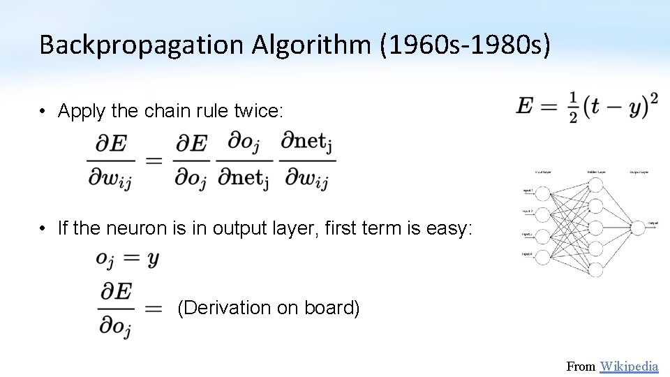
Backpropagation Algorithm (1960 s-1980 s) • Apply the chain rule twice: • If the neuron is in output layer, first term is easy: (Derivation on board) From Wikipedia

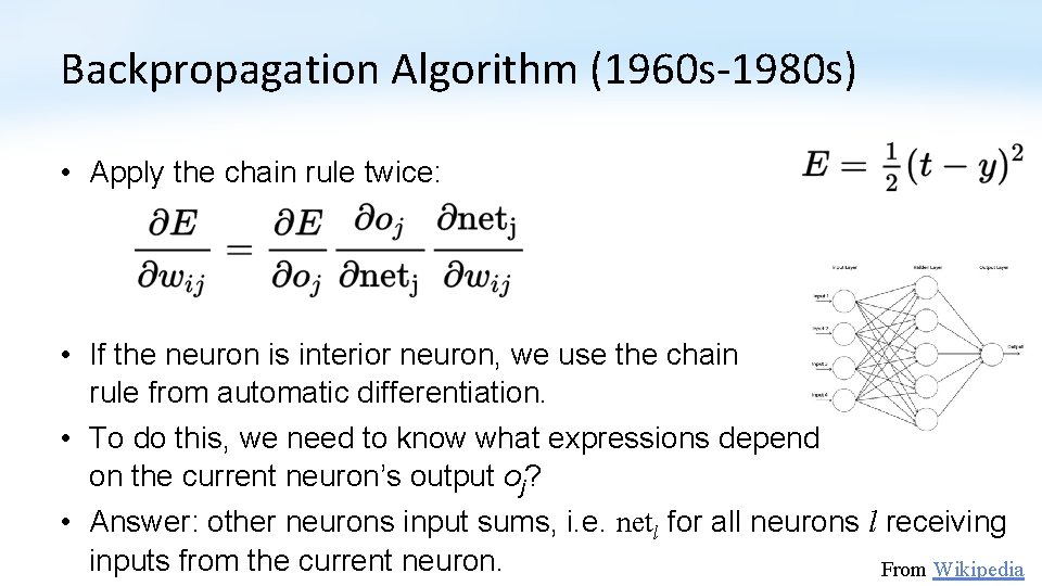
Backpropagation Algorithm (1960 s-1980 s) • Apply the chain rule twice: • If the neuron is interior neuron, we use the chain rule from automatic differentiation. • To do this, we need to know what expressions depend on the current neuron’s output oj? • Answer: other neurons input sums, i. e. netl for all neurons l receiving inputs from the current neuron. From Wikipedia

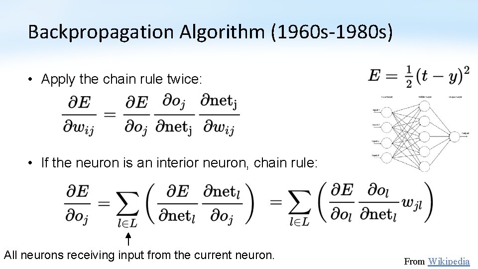
Backpropagation Algorithm (1960 s-1980 s) • Apply the chain rule twice: • If the neuron is an interior neuron, chain rule: All neurons receiving input from the current neuron. From Wikipedia

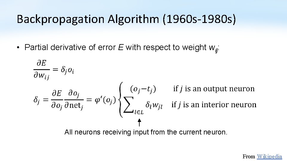
Backpropagation Algorithm (1960 s-1980 s) • Partial derivative of error E with respect to weight wij: All neurons receiving input from the current neuron. From Wikipedia

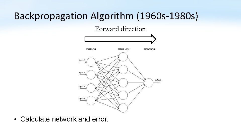
Backpropagation Algorithm (1960 s-1980 s) Forward direction • Calculate network and error.

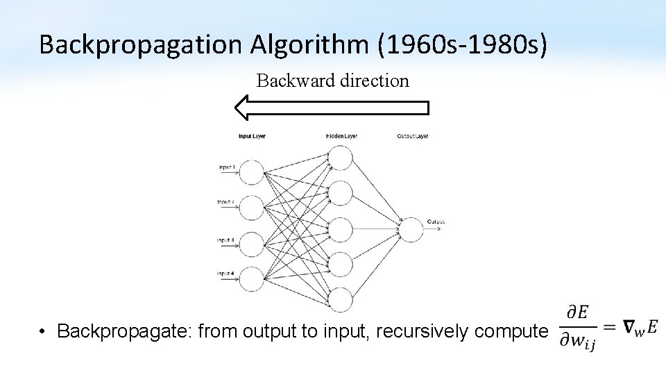
Backpropagation Algorithm (1960 s-1980 s) Backward direction • Backpropagate: from output to input, recursively compute

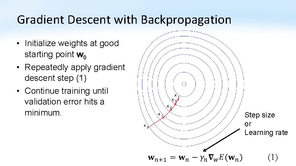
Gradient Descent with Backpropagation • Initialize weights at good starting point w 0 • Repeatedly apply gradient descent step (1) • Continue training until validation error hits a minimum. Step size or Learning rate (1)

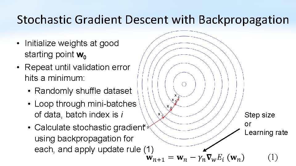
Stochastic Gradient Descent with Backpropagation • Initialize weights at good starting point w 0 • Repeat until validation error hits a minimum: • Randomly shuffle dataset • Loop through mini-batches of data, batch index is i • Calculate stochastic gradient using backpropagation for each, and apply update rule (1) Step size or Learning rate (1)