CS 636 Computer Vision Estimating Parametric and Layered

CS 636 Computer Vision Estimating Parametric and Layered Motion Nathan Jacobs

Overview • Motion fields and parallax • Parametric Motion • Layered Motion

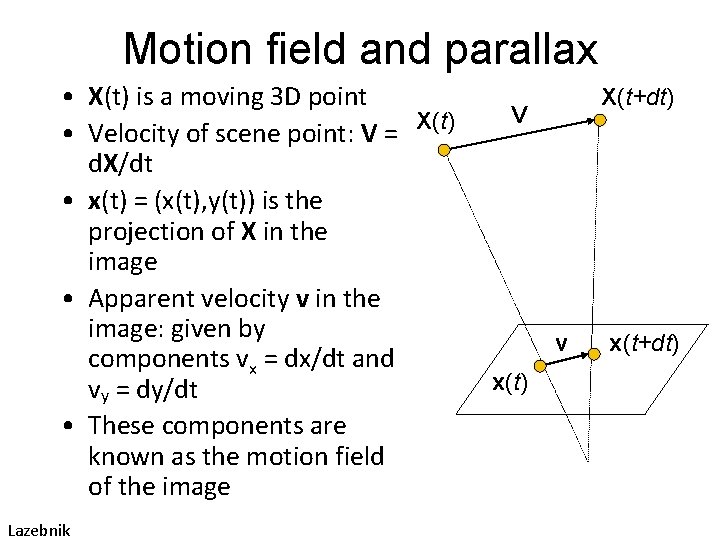
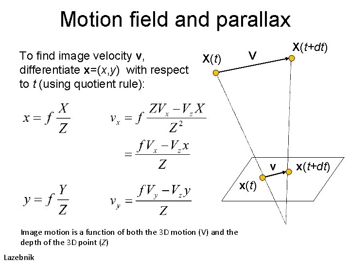
Motion field and parallax • X(t) is a moving 3 D point • Velocity of scene point: V = X(t) d. X/dt • x(t) = (x(t), y(t)) is the projection of X in the image • Apparent velocity v in the image: given by components vx = dx/dt and vy = dy/dt • These components are known as the motion field of the image Lazebnik X(t+dt) V v x(t) x(t+dt)

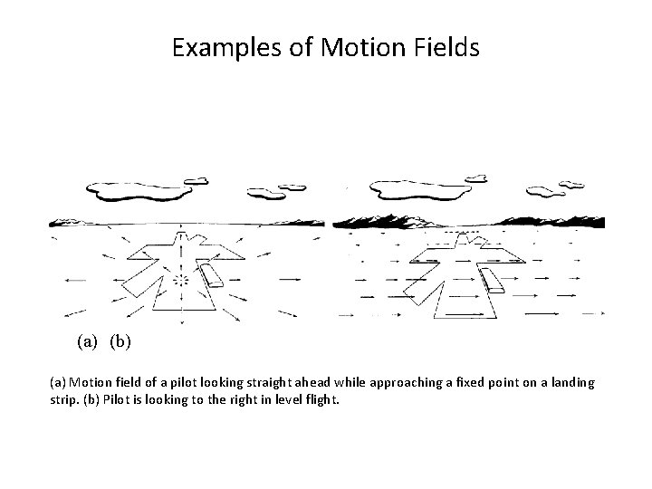
Examples of Motion Fields (a) (b) (a) Motion field of a pilot looking straight ahead while approaching a fixed point on a landing strip. (b) Pilot is looking to the right in level flight.

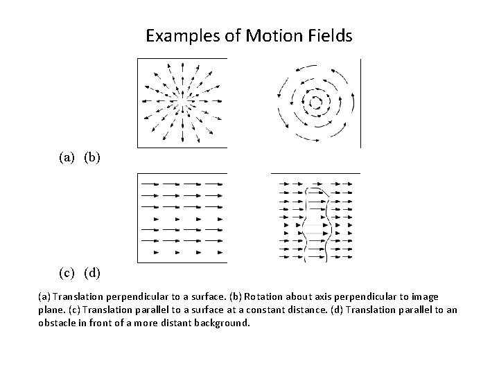
Examples of Motion Fields (a) (b) (c) (d) (a) Translation perpendicular to a surface. (b) Rotation about axis perpendicular to image plane. (c) Translation parallel to a surface at a constant distance. (d) Translation parallel to an obstacle in front of a more distant background.

Motion field and parallax To find image velocity v, differentiate x=(x, y) with respect to t (using quotient rule): X(t) X(t+dt) V v x(t) Image motion is a function of both the 3 D motion (V) and the depth of the 3 D point (Z) Lazebnik x(t+dt)

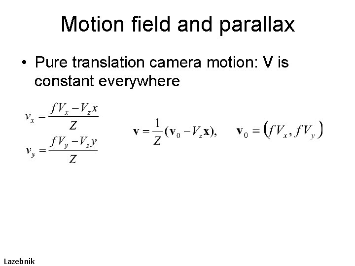
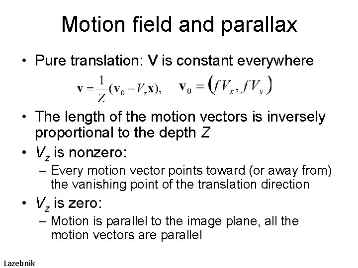
Motion field and parallax • Pure translation camera motion: V is constant everywhere Lazebnik

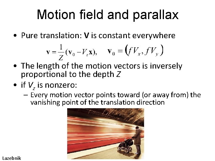
Motion field and parallax • Pure translation: V is constant everywhere • The length of the motion vectors is inversely proportional to the depth Z • if Vz is nonzero: – Every motion vector points toward (or away from) the vanishing point of the translation direction Lazebnik

Motion field and parallax • Pure translation: V is constant everywhere • The length of the motion vectors is inversely proportional to the depth Z • Vz is nonzero: – Every motion vector points toward (or away from) the vanishing point of the translation direction • Vz is zero: – Motion is parallel to the image plane, all the motion vectors are parallel Lazebnik

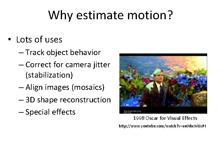
Why estimate motion? • Lots of uses – Track object behavior – Correct for camera jitter (stabilization) – Align images (mosaics) – 3 D shape reconstruction – Special effects 1998 Oscar for Visual Effects http: //www. youtube. com/watch? v=au 0 ibc. WUx. PI

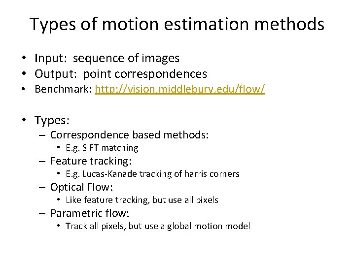
Types of motion estimation methods • Input: sequence of images • Output: point correspondences • Benchmark: http: //vision. middlebury. edu/flow/ • Types: – Correspondence based methods: • E. g. SIFT matching – Feature tracking: • E. g. Lucas-Kanade tracking of harris corners – Optical Flow: • Like feature tracking, but use all pixels – Parametric flow: • Track all pixels, but use a global motion model

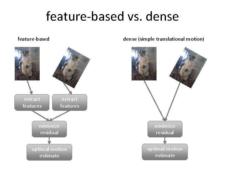
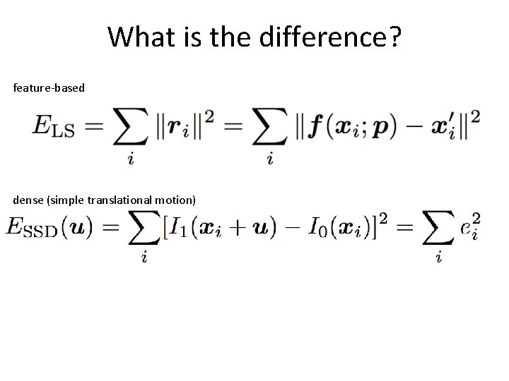
feature-based vs. dense feature-based extract features dense (simple translational motion) extract features minimize residual optimal motion estimate

What is the difference? feature-based dense (simple translational motion)

Discussion: features vs. flow? • Features are better for: • Flow is better for:

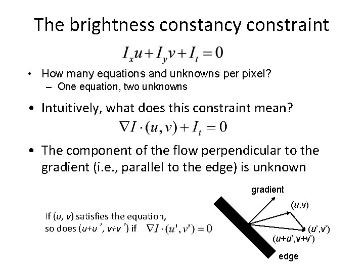
The brightness constancy constraint • How many equations and unknowns per pixel? – One equation, two unknowns • Intuitively, what does this constraint mean? • The component of the flow perpendicular to the gradient (i. e. , parallel to the edge) is unknown gradient If (u, v) satisfies the equation, so does (u+u’, v+v’) if (u, v) (u’, v’) (u+u’, v+v’) edge

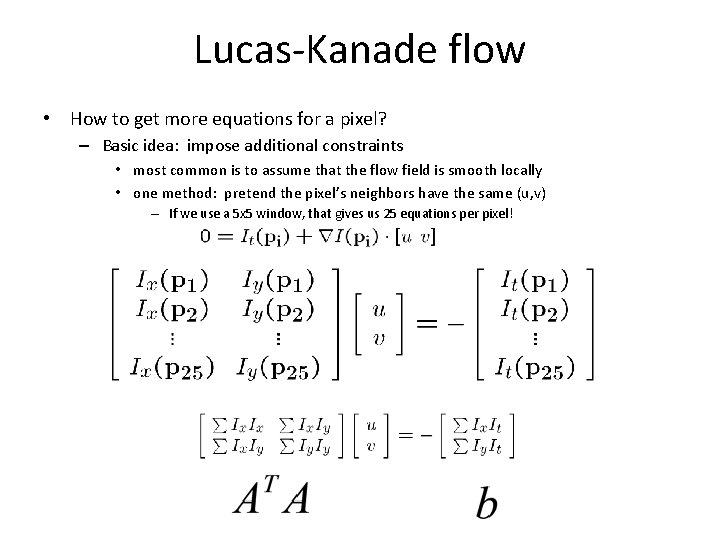
Lucas-Kanade flow • How to get more equations for a pixel? – Basic idea: impose additional constraints • most common is to assume that the flow field is smooth locally • one method: pretend the pixel’s neighbors have the same (u, v) – If we use a 5 x 5 window, that gives us 25 equations per pixel!

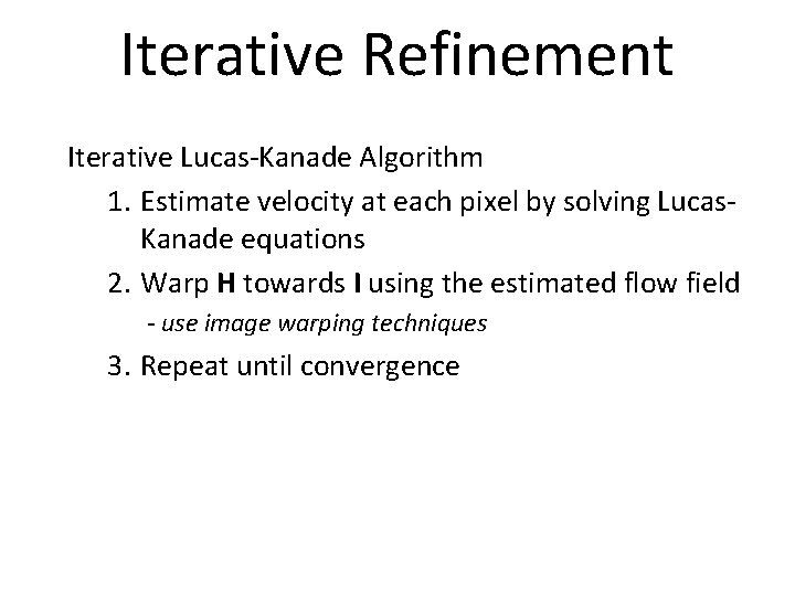
Iterative Refinement Iterative Lucas-Kanade Algorithm 1. Estimate velocity at each pixel by solving Lucas. Kanade equations 2. Warp H towards I using the estimated flow field - use image warping techniques 3. Repeat until convergence

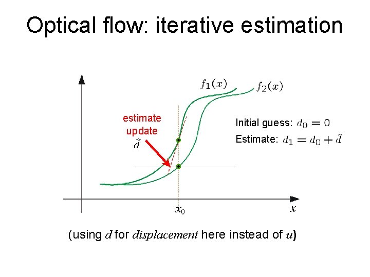
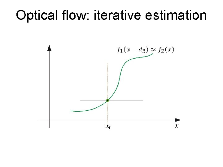
Optical flow: iterative estimation estimate update Initial guess: Estimate: x 0 x (using d for displacement here instead of u)

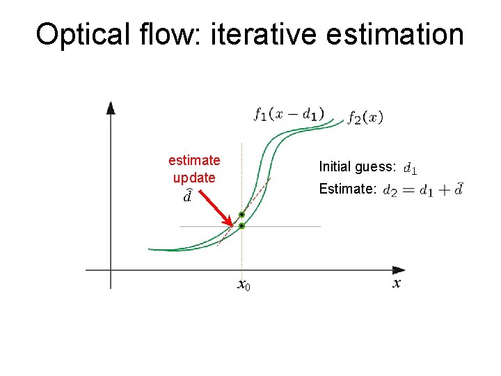
Optical flow: iterative estimation estimate update Initial guess: Estimate: x 0 x

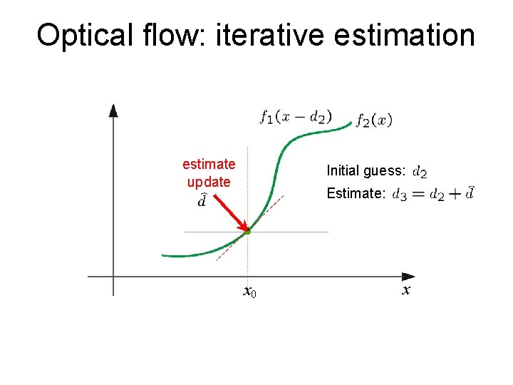
Optical flow: iterative estimation estimate update Initial guess: Estimate: x 0 x

Optical flow: iterative estimation x 0 x

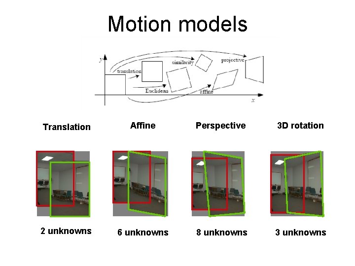
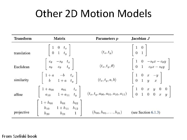
Motion models Translation Affine Perspective 3 D rotation 2 unknowns 6 unknowns 8 unknowns 3 unknowns

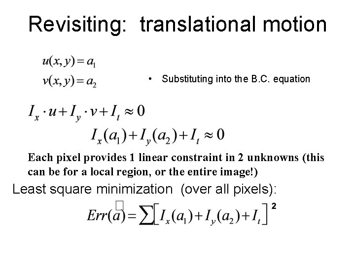
Revisiting: translational motion • Substituting into the B. C. equation Each pixel provides 1 linear constraint in 2 unknowns (this can be for a local region, or the entire image!) Least square minimization (over all pixels):

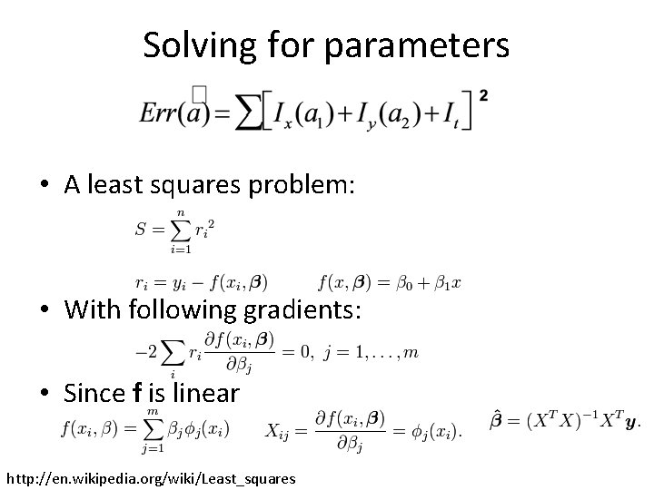
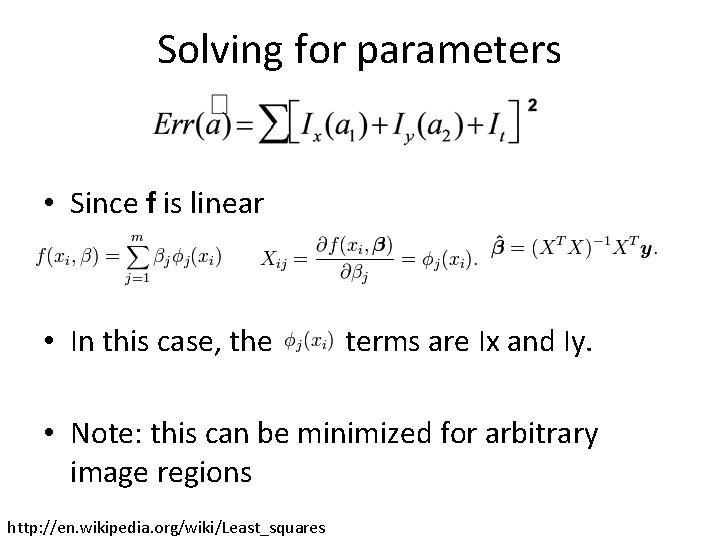
Solving for parameters • A least squares problem: • With following gradients: • Since f is linear http: //en. wikipedia. org/wiki/Least_squares

Solving for parameters • Since f is linear • In this case, the terms are Ix and Iy. • Note: this can be minimized for arbitrary image regions http: //en. wikipedia. org/wiki/Least_squares

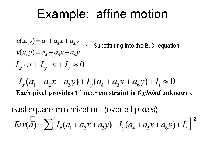
Example: affine motion • Substituting into the B. C. equation Each pixel provides 1 linear constraint in 6 global unknowns Least square minimization (over all pixels):

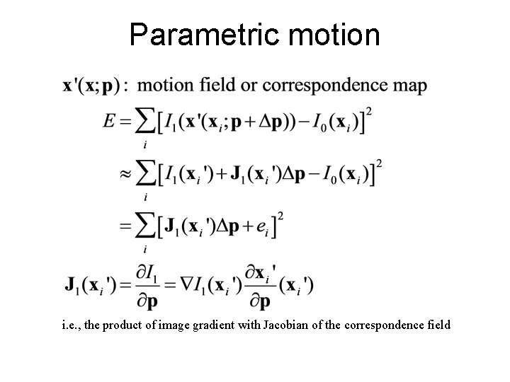
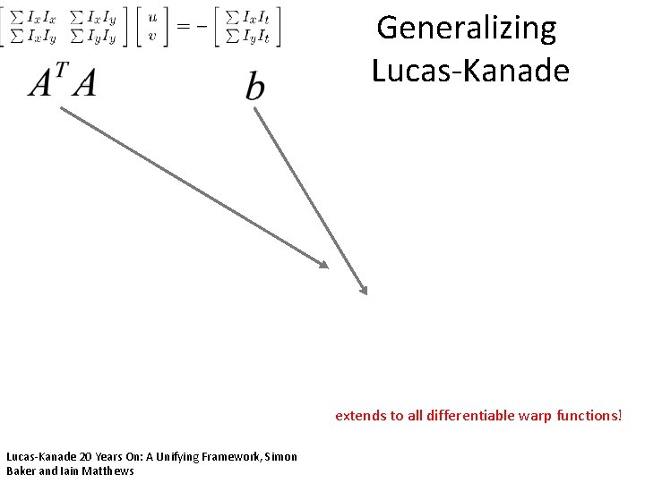
Parametric motion i. e. , the product of image gradient with Jacobian of the correspondence field

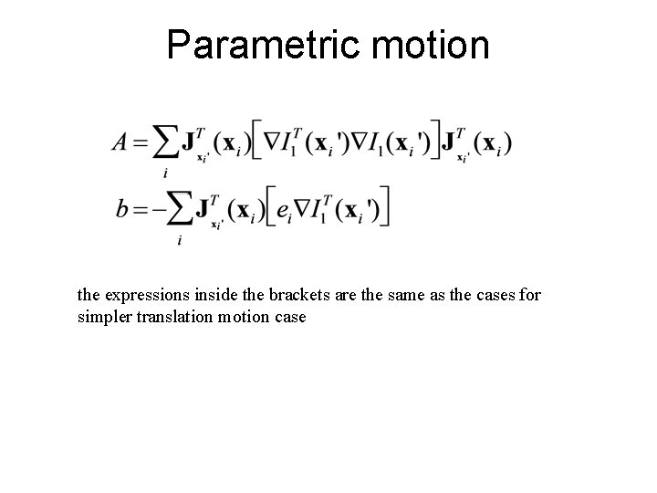
Parametric motion the expressions inside the brackets are the same as the cases for simpler translation motion case

Other 2 D Motion Models From Szeliski book

Generalizing Lucas-Kanade extends to all differentiable warp functions! Lucas-Kanade 20 Years On: A Unifying Framework, Simon Baker and Iain Matthews

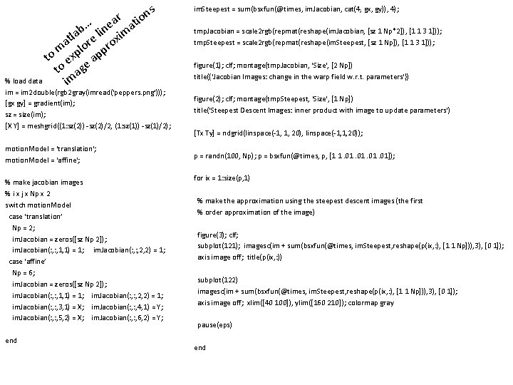
s n o ti ar a e … lab e lin xim t a lor ro m p to exp ap to age im % load data im = im 2 double(rgb 2 gray(imread('peppers. png'))); [gx gy] = gradient(im); sz = size(im); [X Y] = meshgrid((1: sz(2)) -sz(2)/2, (1: sz(1)) -sz(1)/2); motion. Model = 'translation'; motion. Model = 'affine'; % make jacobian images % i x j x Np x 2 switch motion. Model case 'translation’ Np = 2; im. Jacobian = zeros([sz Np 2]); im. Jacobian(: , 1, 1) = 1; im. Jacobian(: , 2, 2) = 1; case 'affine’ Np = 6; im. Jacobian = zeros([sz Np 2]); im. Jacobian(: , 1, 1) = 1; im. Jacobian(: , 2, 2) = 1; im. Jacobian(: , 3, 1) = X; im. Jacobian(: , 4, 1) = Y; im. Jacobian(: , 5, 2) = X; im. Jacobian(: , 6, 2) = Y; end im. Steepest = sum(bsxfun(@times, im. Jacobian, cat(4, gx, gy)), 4); tmp. Jacobian = scale 2 rgb(repmat(reshape(im. Jacobian, [sz 1 Np*2]), [1 1 3 1])); tmp. Steepest = scale 2 rgb(repmat(reshape(im. Steepest, [sz 1 Np]), [1 1 3 1])); figure(1); clf; montage(tmp. Jacobian, 'Size', [2 Np]) title({'Jacobian Images: change in the warp field w. r. t. parameters'}) figure(2); clf; montage(tmp. Steepest, 'Size', [1 Np]) title('Steepest Descent Images: inner product with image to update parameters') [Tx Ty] = ndgrid(linspace(-1, 1, 20), linspace(-1, 1, 20)); p = randn(100, Np); p = bsxfun(@times, p, [1 1. 01. 01]); for ix = 1: size(p, 1) % make the approximation using the steepest descent images (the first % order approximation of the image) figure(3); clf; subplot(121); imagesc(im + sum(bsxfun(@times, im. Steepest, reshape(p(ix, : ), [1 1 Np])), 3), [0 1]); axis image off; title(p(ix, : )) subplot(122) imagesc(im + sum(bsxfun(@times, im. Steepest, reshape(p(ix, : ), [1 1 Np])), 3), [0 1]); axis image off; xlim([40 100]), ylim([160 210]); colormap gray pause(eps) end

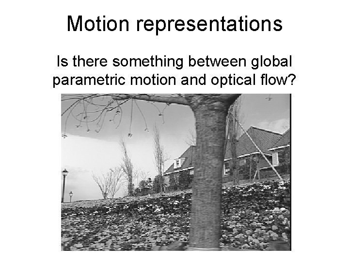
Motion representations Is there something between global parametric motion and optical flow?

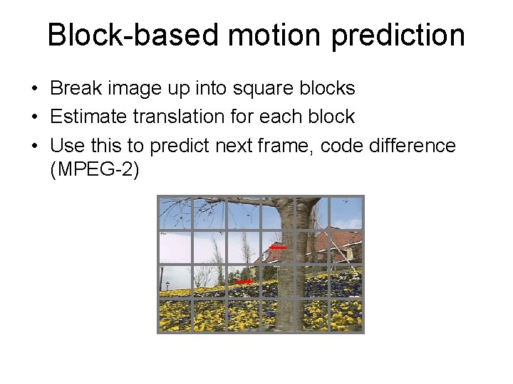
Block-based motion prediction • Break image up into square blocks • Estimate translation for each block • Use this to predict next frame, code difference (MPEG-2)

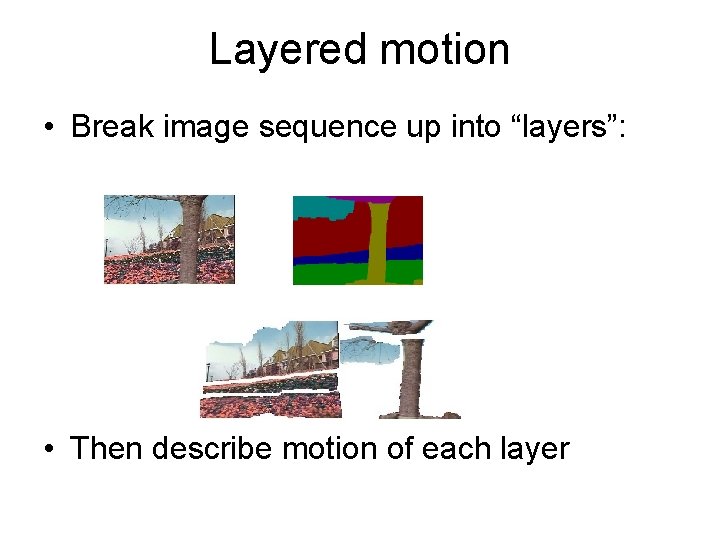
Layered motion • Break image sequence up into “layers”: = • Then describe motion of each layer

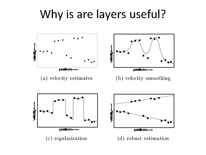
Layered motion • Advantages: – can represent occlusions / dis-occlusions – each layer’s motion can be smooth – video segmentation for semantic processing • Difficulties: – how do we determine the correct number? – how do we assign pixels? – how do we model the motion?

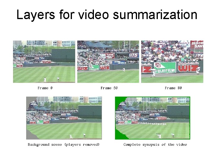
Layers for video summarization

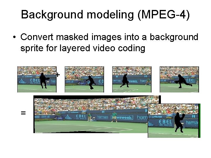
Background modeling (MPEG-4) • Convert masked images into a background sprite for layered video coding ++ = + +

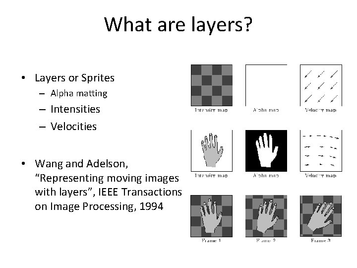
What are layers? • Layers or Sprites – Alpha matting – Intensities – Velocities • Wang and Adelson, “Representing moving images with layers”, IEEE Transactions on Image Processing, 1994

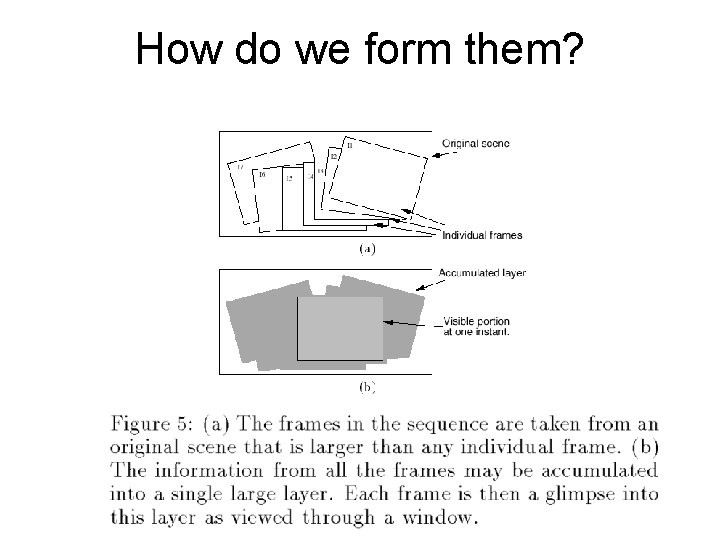
How do we form them?

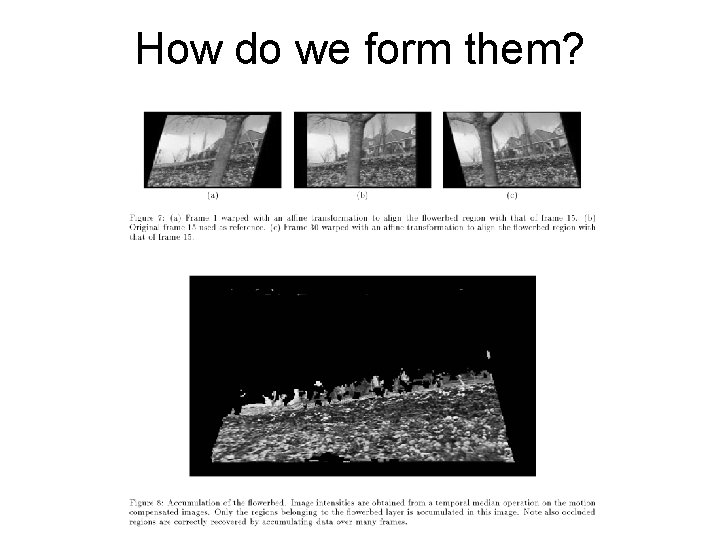
How do we form them?

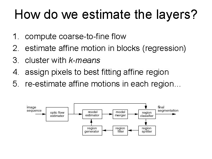
How do we estimate the layers? 1. 2. 3. 4. 5. compute coarse-to-fine flow estimate affine motion in blocks (regression) cluster with k-means assign pixels to best fitting affine region re-estimate affine motions in each region…

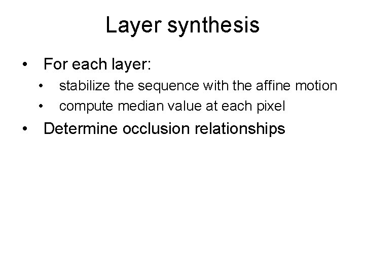
Layer synthesis • For each layer: • • stabilize the sequence with the affine motion compute median value at each pixel • Determine occlusion relationships

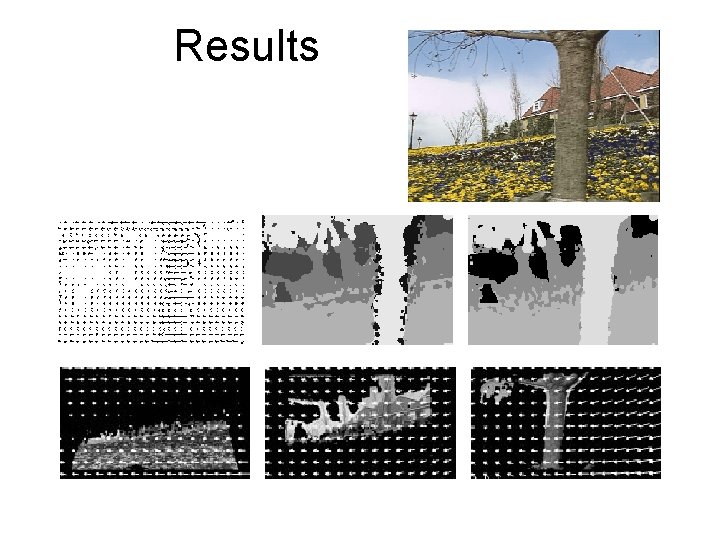
Results

Why is are layers useful?

summary • parametric motion: generalized Lucas-Kanade • layered motion models