CS 6045 Advanced Algorithms Sorting Algorithms Review Insertion

CS 6045: Advanced Algorithms Sorting Algorithms

Review • Insertion Sort – Time complexity – Space complexity • Merge Sort – Time complexity – Space complexity • Comparisons

Review: Solving Recurrences • Substitution method • Iteration method • Master method

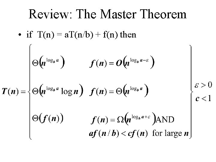
Review: The Master Theorem • if T(n) = a. T(n/b) + f(n) then

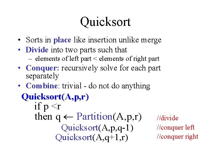
Quicksort • Sorts in place like insertion unlike merge • Divide into two parts such that – elements of left part < elements of right part • Conquer: recursively solve for each part separately • Combine: trivial - do not do anything Quicksort(A, p, r) if p <r then q Partition(A, p, r) Quicksort(A, p, q-1) Quicksort(A, q+1, r) //divide //conquer left //conquer right

Quicksort • Another divide-and-conquer algorithm – The array A[p. . r] is partitioned into two nonempty subarrays A[p. . q] and A[q+1. . r] • Invariant: All elements in A[p. . q] are less than all elements in A[q+1. . r] – The subarrays are recursively sorted by calls to quicksort – Unlike merge sort, no combining step: two subarrays form an already-sorted array

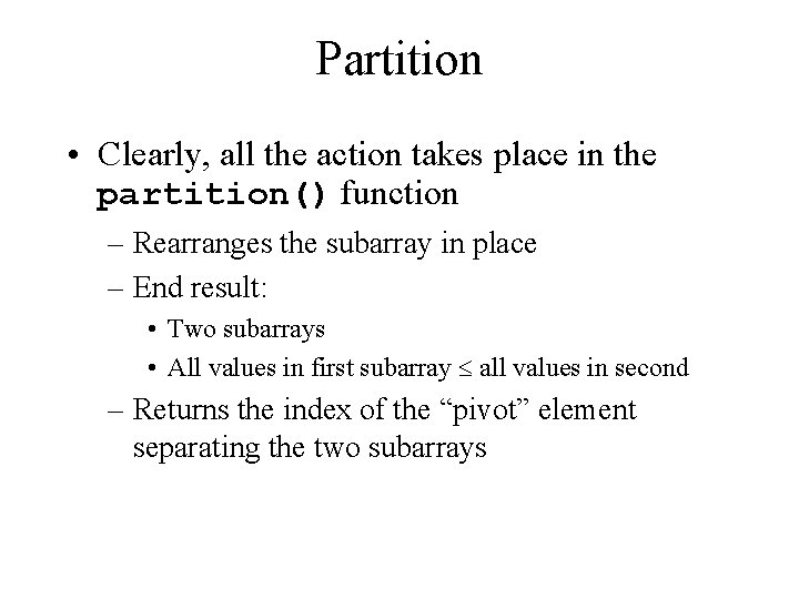
Partition • Clearly, all the action takes place in the partition() function – Rearranges the subarray in place – End result: • Two subarrays • All values in first subarray all values in second – Returns the index of the “pivot” element separating the two subarrays

Divide = Partition PARTITION(A, p, r) //Partition array from A[p] to A[r] with pivot A[r] //Result: All elements original A[r] has index i x = A[r] i =p-1 for j = p to r - 1 if A[j] <= x i=i+1 exchange A[i] A[j] exchange A[i+1] with A[r] return i + 1

PARTITION(A, p, r) x = A[r] i =p-1 for j = p to r - 1 if A[j] <= x i=i+1 exchange A[i] A[j] exchange A[i+1] with A[r] return i + 1

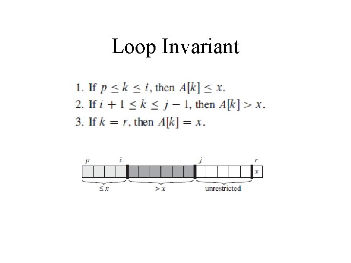
Loop Invariant

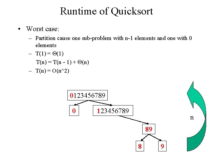
Runtime of Quicksort • Worst case: – Partition cause one sub-problem with n-1 elements and one with 0 elements – T(1) = (1) T(n) = T(n - 1) + (n) – T(n) = O(n^2) 0123456789 0 123456789 n 89 8 9

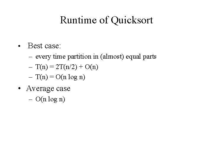
Runtime of Quicksort • Best case: – every time partition in (almost) equal parts – T(n) = 2 T(n/2) + O(n) – T(n) = O(n log n) • Average case – O(n log n)

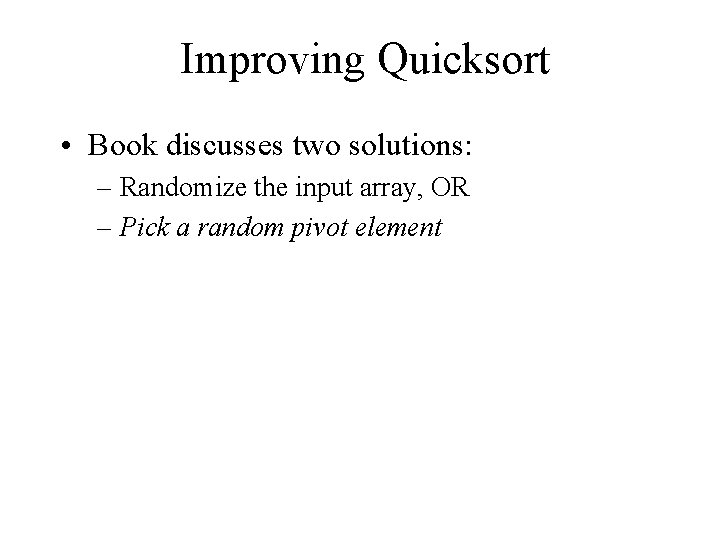
Improving Quicksort • Book discusses two solutions: – Randomize the input array, OR – Pick a random pivot element

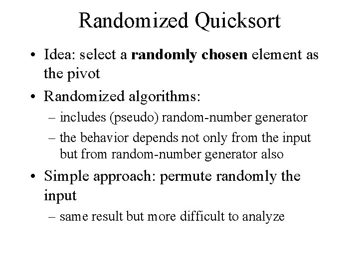
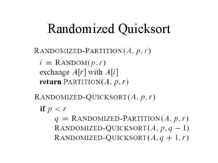
Randomized Quicksort • Idea: select a randomly chosen element as the pivot • Randomized algorithms: – includes (pseudo) random-number generator – the behavior depends not only from the input but from random-number generator also • Simple approach: permute randomly the input – same result but more difficult to analyze

Randomized Quicksort

Randomized Quicksort • Partition around first element: O(n^2) worst -case • Average case: O(n log n)

Heap Sort • So far we’ve talked about three algorithms to sort an array of numbers – What is the advantage of merge sort? – What is the advantage of insertion sort? – What is the advantage of quick sort? • Heap sort

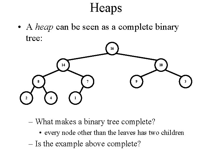
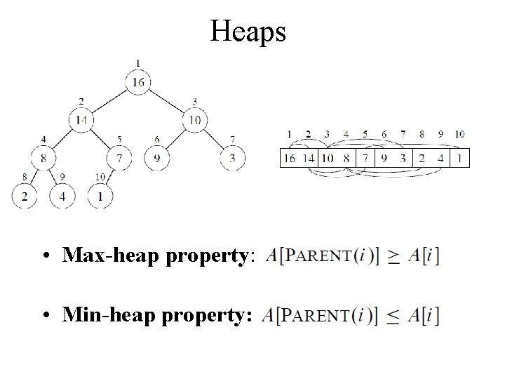
Heaps • A heap can be seen as a complete binary tree: 16 14 10 8 2 7 4 9 1 – What makes a binary tree complete? • every node other than the leaves has two children – Is the example above complete? 3

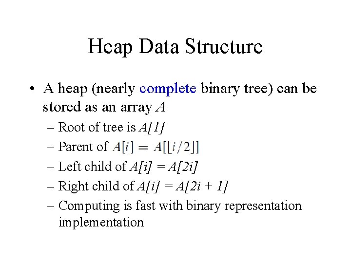
Heap Data Structure • A heap (nearly complete binary tree) can be stored as an array A – Root of tree is A[1] – Parent of – Left child of A[i] = A[2 i] – Right child of A[i] = A[2 i + 1] – Computing is fast with binary representation implementation

Heaps • Max-heap property: • Min-heap property:

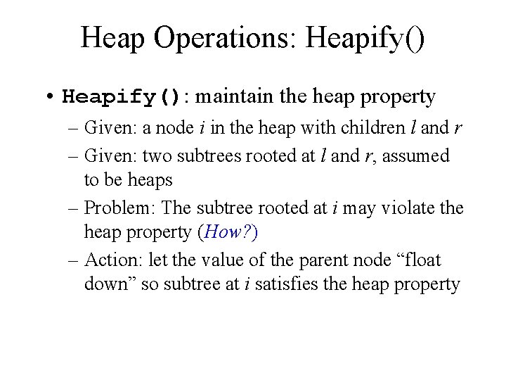
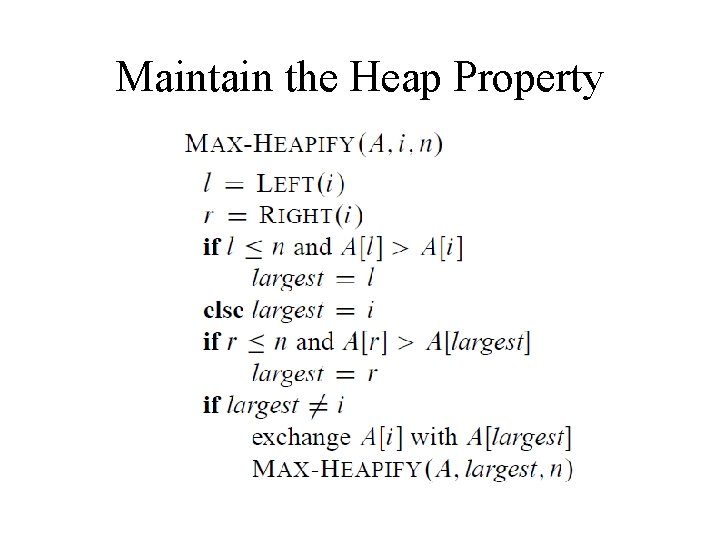
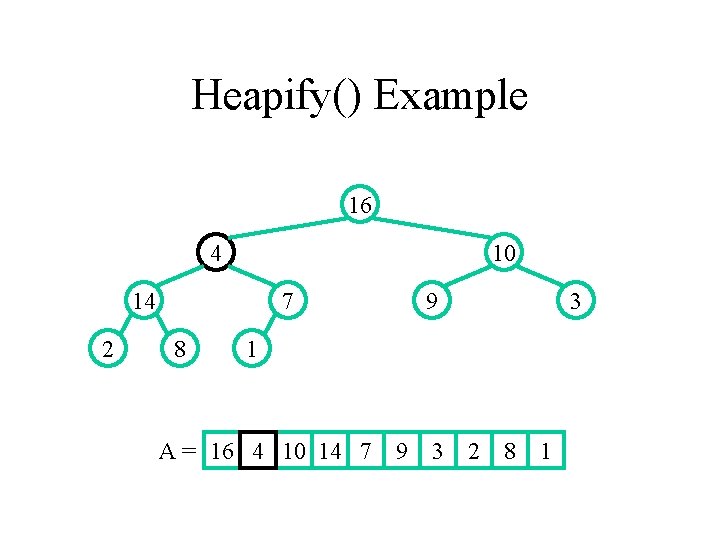
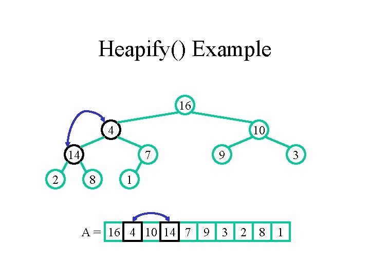
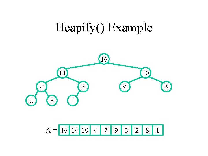
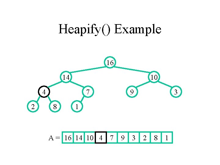
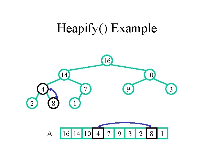
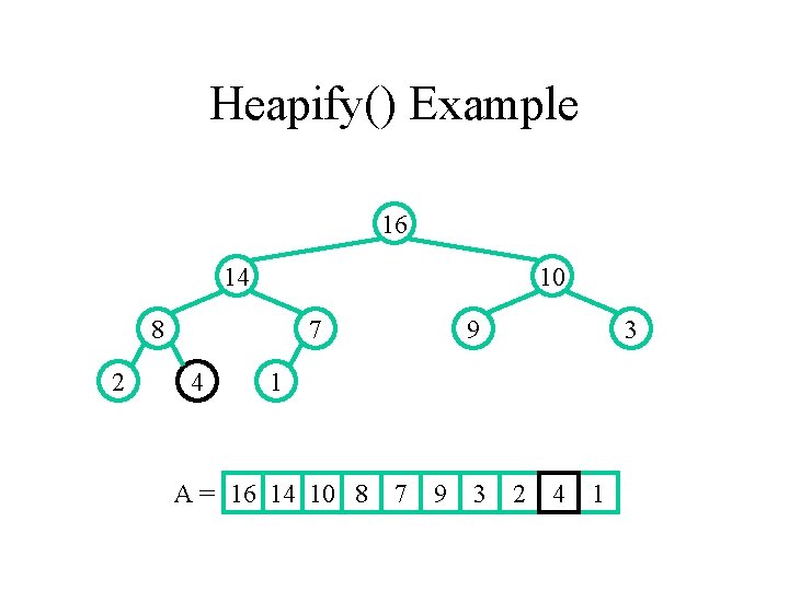
Heap Operations: Heapify() • Heapify(): maintain the heap property – Given: a node i in the heap with children l and r – Given: two subtrees rooted at l and r, assumed to be heaps – Problem: The subtree rooted at i may violate the heap property (How? ) – Action: let the value of the parent node “float down” so subtree at i satisfies the heap property

Maintain the Heap Property

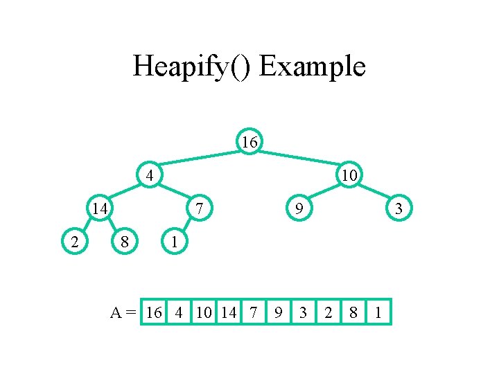
Heapify() Example 16 4 10 14 2 7 8 9 3 1 A = 16 4 10 14 7 9 3 2 8 1

Heapify() Example 16 4 10 14 2 7 8 9 3 1 A = 16 4 10 14 7 9 3 2 8 1

Heapify() Example 16 4 10 14 2 7 8 9 3 1 A = 16 4 10 14 7 9 3 2 8 1

Heapify() Example 16 14 10 4 2 7 8 9 3 1 A = 16 14 10 4 7 9 3 2 8 1

Heapify() Example 16 14 10 4 2 7 8 9 3 1 A = 16 14 10 4 7 9 3 2 8 1

Heapify() Example 16 14 10 4 2 7 8 9 3 1 A = 16 14 10 4 7 9 3 2 8 1

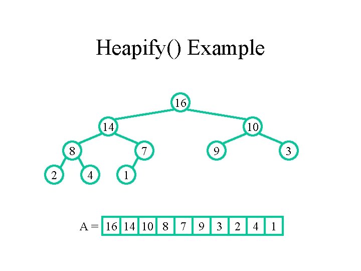
Heapify() Example 16 14 10 8 2 7 4 9 3 1 A = 16 14 10 8 7 9 3 2 4 1

Heapify() Example 16 14 10 8 2 7 4 9 3 1 A = 16 14 10 8 7 9 3 2 4 1

Heapify() Example 16 14 10 8 2 7 4 9 3 1 A = 16 14 10 8 7 9 3 2 4 1

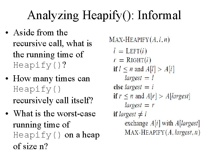
Analyzing Heapify(): Informal • Aside from the recursive call, what is the running time of Heapify()? • How many times can Heapify() recursively call itself? • What is the worst-case running time of Heapify() on a heap of size n?

Analyzing Heapify(): Formal • Fixing up relationships between i, l, and r takes (1) time • If the heap at i has n elements, how many elements can the subtrees at l or r have? – Answer: 2 n/3 (worst case: bottom row 1/2 full) • So time taken by Heapify() is given by T(n) T(2 n/3) + (1)

Analyzing Heapify(): Formal • So we have T(n) T(2 n/3) + (1) • By case 2 of the Master Theorem, T(n) = O(log n)

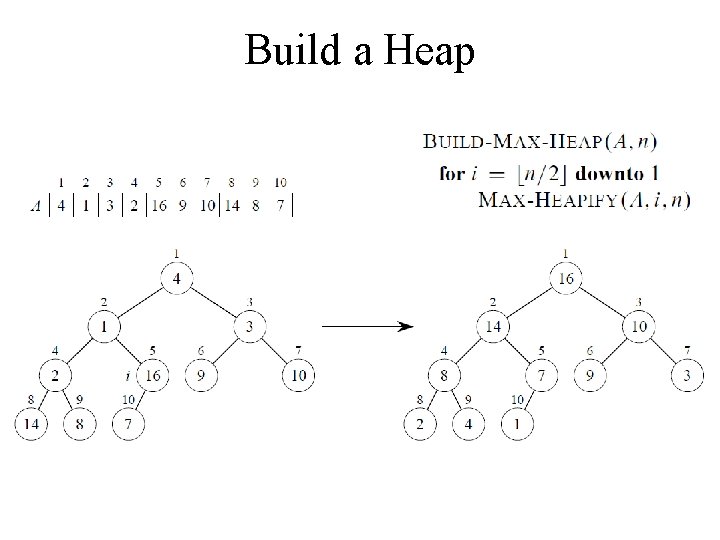
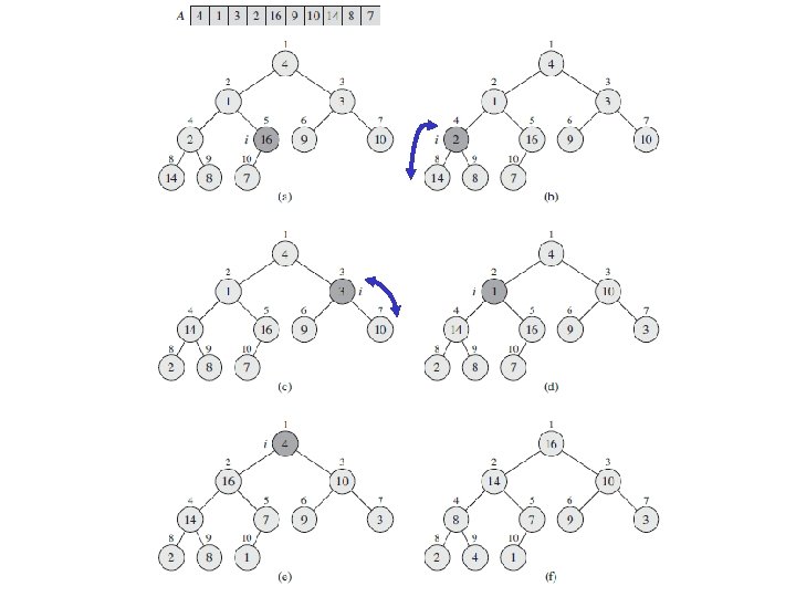
Heap Operations: Build. Heap() • We can build a heap in a bottom-up manner by running Heapify() on successive subarrays – Fact: for array of length n, all elements in range A[ n/2 + 1. . n] are heaps (Why? ) – So: • Walk backwards through the array from n/2 to 1, calling Heapify() on each node. • Order of processing guarantees that the children of node i are heaps when i is processed

Build a Heap

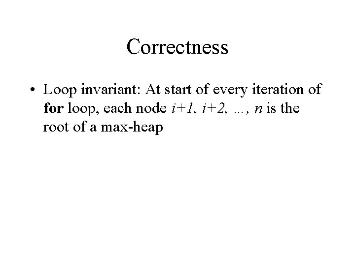
Correctness • Loop invariant: At start of every iteration of for loop, each node i+1, i+2, …, n is the root of a max-heap

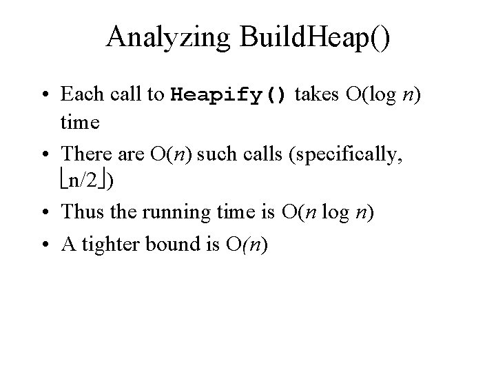
Analyzing Build. Heap() • Each call to Heapify() takes O(log n) time • There are O(n) such calls (specifically, n/2 ) • Thus the running time is O(n log n) • A tighter bound is O(n)

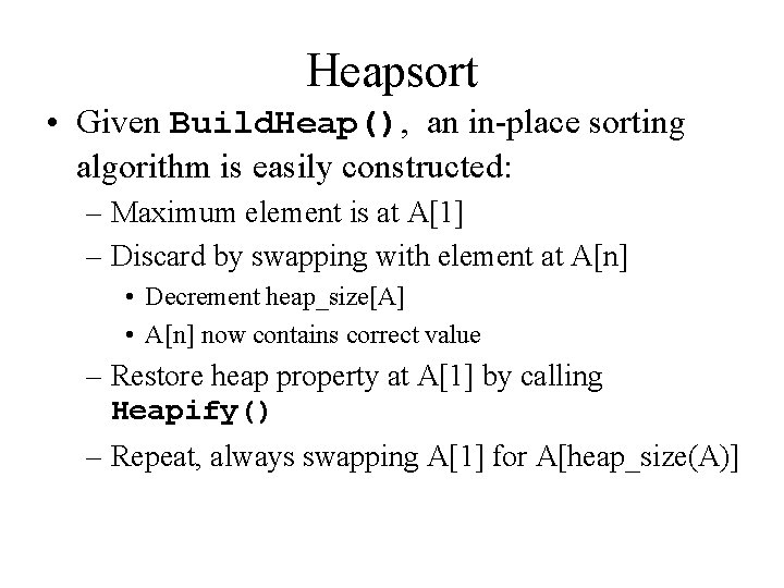
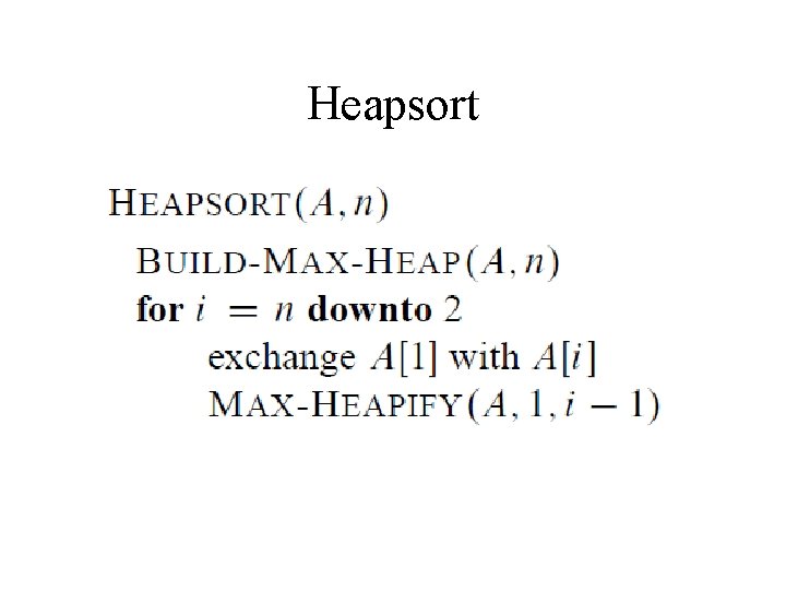
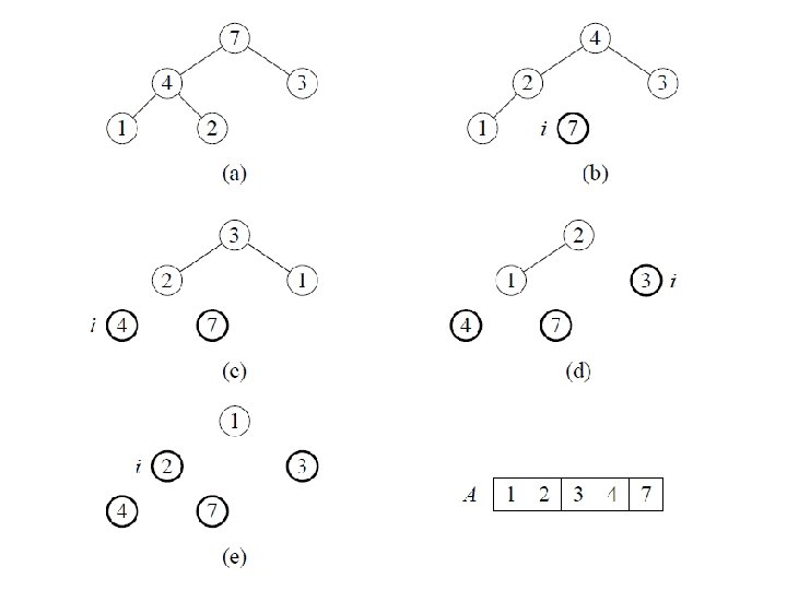
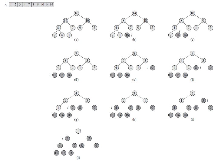
Heapsort • Given Build. Heap(), an in-place sorting algorithm is easily constructed: – Maximum element is at A[1] – Discard by swapping with element at A[n] • Decrement heap_size[A] • A[n] now contains correct value – Restore heap property at A[1] by calling Heapify() – Repeat, always swapping A[1] for A[heap_size(A)]

Heapsort

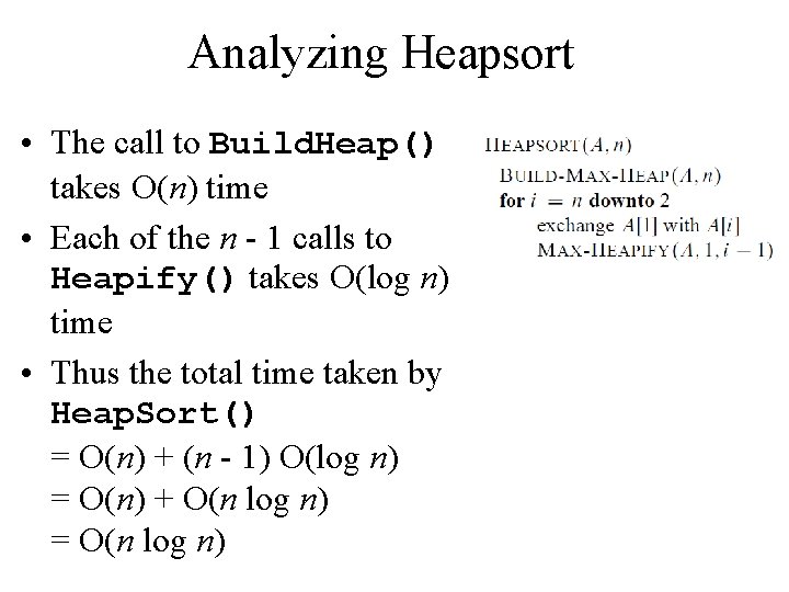
Analyzing Heapsort • The call to Build. Heap() takes O(n) time • Each of the n - 1 calls to Heapify() takes O(log n) time • Thus the total time taken by Heap. Sort() = O(n) + (n - 1) O(log n) = O(n) + O(n log n) = O(n log n)

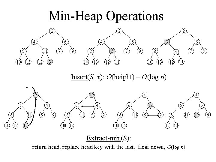
Min-Heap Operations 2 2 4 8 6 11 10 13 7 4 9 6 8 3 12 2 10 3 13 12 7 6 3 9 8 11 10 7 4 13 12 9 11 Insert(S, x): O(height) = O(log n) 2 12 6 8 10 13 4 11 12 5 6 9 8 10 13 4 4 11 5 6 9 8 10 13 4 12 11 5 6 9 8 5 11 10 13 Extract-min(S): return head, replace head key with the last, float down, O(log n) 12 9

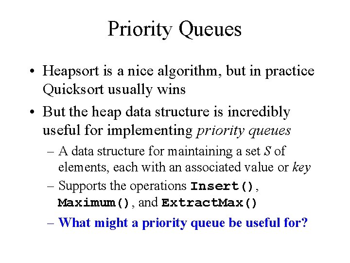
Priority Queues • Heapsort is a nice algorithm, but in practice Quicksort usually wins • But the heap data structure is incredibly useful for implementing priority queues – A data structure for maintaining a set S of elements, each with an associated value or key – Supports the operations Insert(), Maximum(), and Extract. Max() – What might a priority queue be useful for?

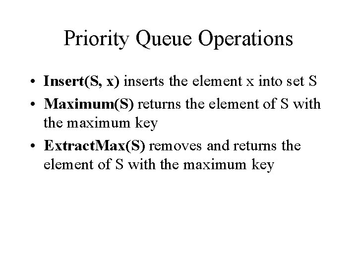
Priority Queue Operations • Insert(S, x) inserts the element x into set S • Maximum(S) returns the element of S with the maximum key • Extract. Max(S) removes and returns the element of S with the maximum key

Priority Queues • Applications – job scheduling on shared computer – Dijkstra’s finding shortest paths in graphs – Prim’s algorithm for minimum spanning tree