CS 6045 Advanced Algorithms Data Structures Dynamic Sets

CS 6045: Advanced Algorithms Data Structures

Dynamic Sets • Dynamic sets: – Can grow, shrink (manipulated by algorithms) – Change over time • Dictionary: – Insert/delete elements – Test membership

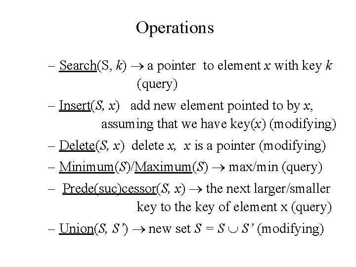
Operations – Search(S, k) a pointer to element x with key k (query) – Insert(S, x) add new element pointed to by x, assuming that we have key(x) (modifying) – Delete(S, x) delete x, x is a pointer (modifying) – Minimum(S)/Maximum(S) max/min (query) – Prede(suc)cessor(S, x) the next larger/smaller key to the key of element x (query) – Union(S, S’) new set S = S S’ (modifying)

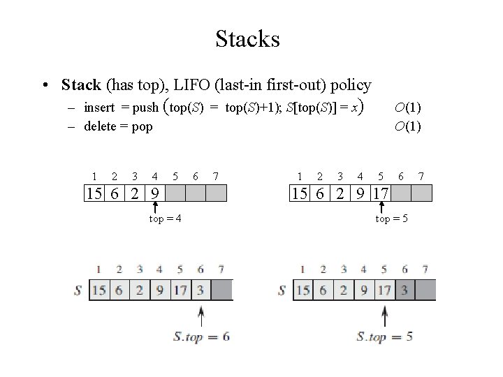
Stacks • Stack (has top), LIFO (last-in first-out) policy – insert = push (top(S) = top(S)+1); S[top(S)] = x) – delete = pop 1 2 3 4 5 15 6 2 9 top = 4 6 7 1 2 3 4 O(1) 5 6 15 6 2 9 17 top = 5 7

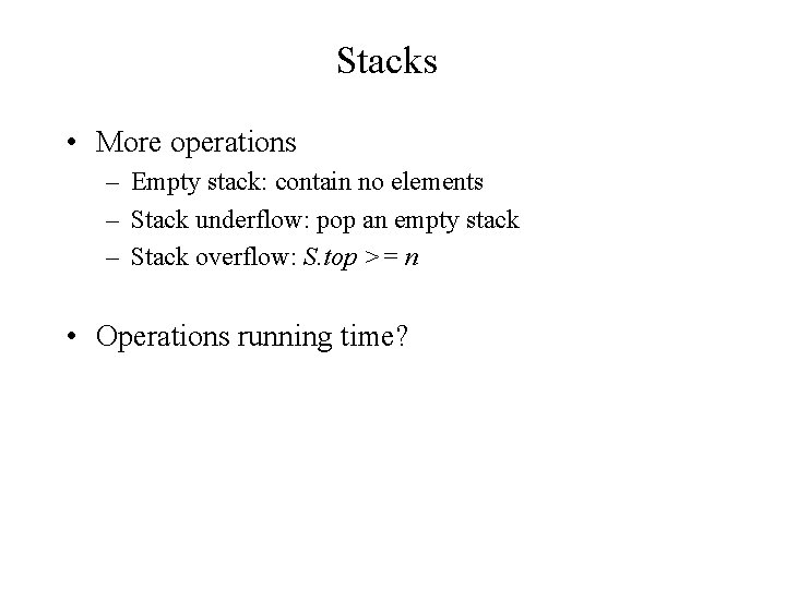
Stacks • More operations – Empty stack: contain no elements – Stack underflow: pop an empty stack – Stack overflow: S. top >= n • Operations running time?

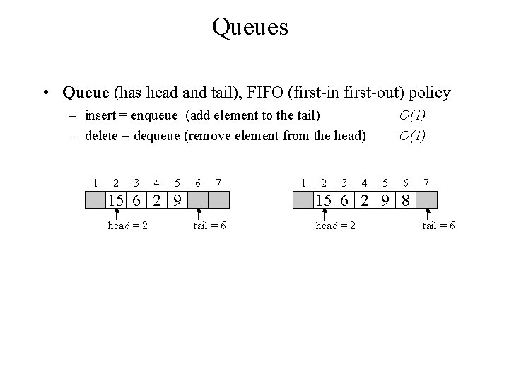
Queues • Queue (has head and tail), FIFO (first-in first-out) policy – insert = enqueue (add element to the tail) – delete = dequeue (remove element from the head) 1 2 3 4 5 6 7 15 6 2 9 head = 2 1 2 3 4 O(1) 5 6 7 15 6 2 9 8 tail = 6 head = 2 tail = 6

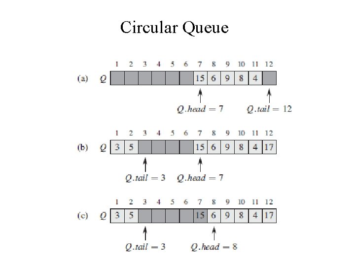
Circular Queue

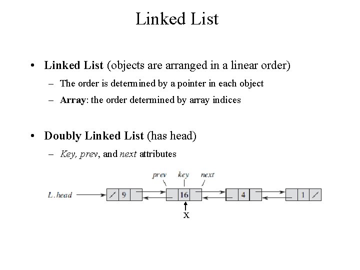
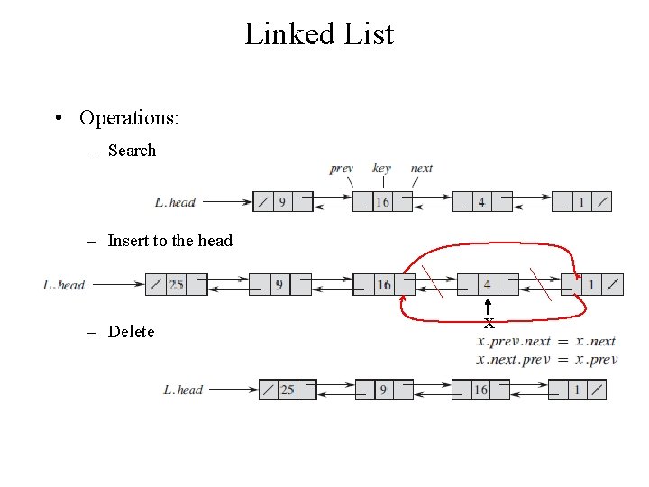
Linked List • Linked List (objects are arranged in a linear order) – The order is determined by a pointer in each object – Array: the order determined by array indices • Doubly Linked List (has head) – Key, prev, and next attributes x

Linked List • Operations: – Search – Insert to the head – Delete x

Linked List • Running time of linked list operations: – Search – Insert – Delete

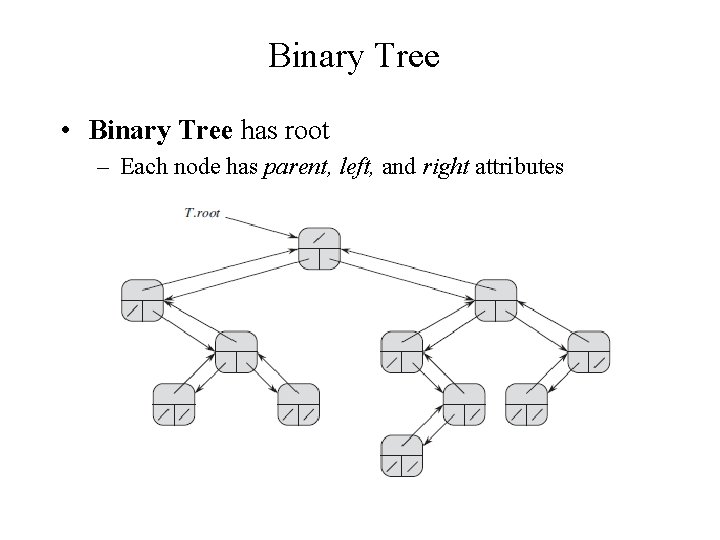
Binary Tree • Binary Tree has root – Each node has parent, left, and right attributes

Binary Search Trees • Binary Search Trees (BSTs) are an important data structure for dynamic sets • Elements have: – – key: an identifying field inducing a total ordering left: pointer to a left child (may be NULL) right: pointer to a right child (may be NULL) p: pointer to a parent node (NULL for root)

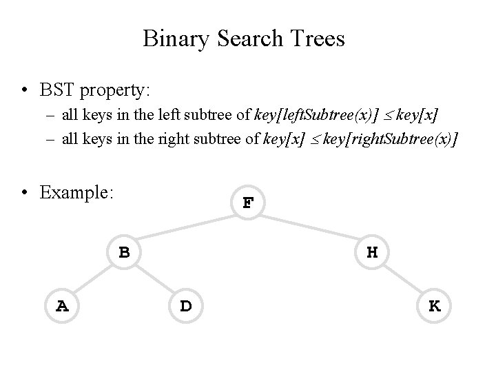
Binary Search Trees • BST property: – all keys in the left subtree of key[left. Subtree(x)] key[x] – all keys in the right subtree of key[x] key[right. Subtree(x)] • Example: F B A H D K

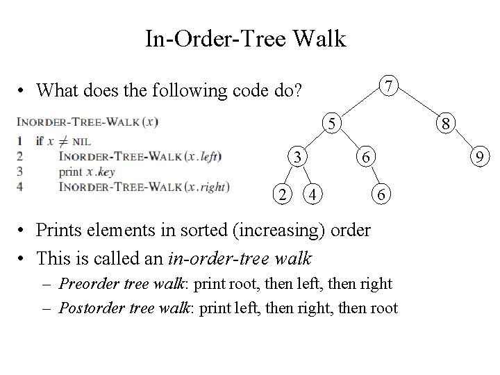
In-Order-Tree Walk 7 • What does the following code do? 5 3 2 8 6 4 9 6 • Prints elements in sorted (increasing) order • This is called an in-order-tree walk – Preorder tree walk: print root, then left, then right – Postorder tree walk: print left, then right, then root

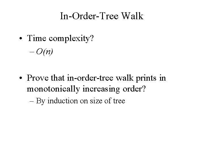
In-Order-Tree Walk • Time complexity? – O(n) • Prove that in-order-tree walk prints in monotonically increasing order? – By induction on size of tree

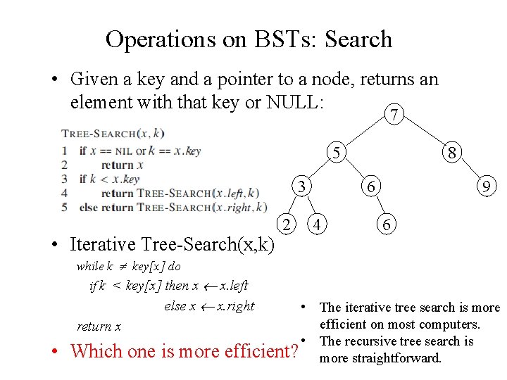
Operations on BSTs: Search • Given a key and a pointer to a node, returns an element with that key or NULL: 7 5 3 • Iterative Tree-Search(x, k) 2 8 6 4 9 6 while k key[x] do if k < key[x] then x x. left else x x. right return x • Which one is more • The iterative tree search is more efficient on most computers. • The recursive tree search is efficient? more straightforward.

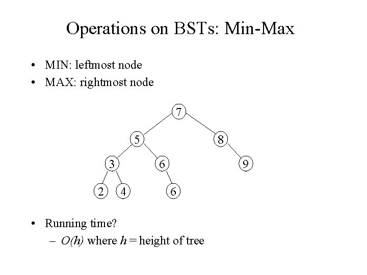
Operations on BSTs: Min-Max • MIN: leftmost node • MAX: rightmost node 7 5 3 2 8 6 4 9 6 • Running time? – O(h) where h = height of tree

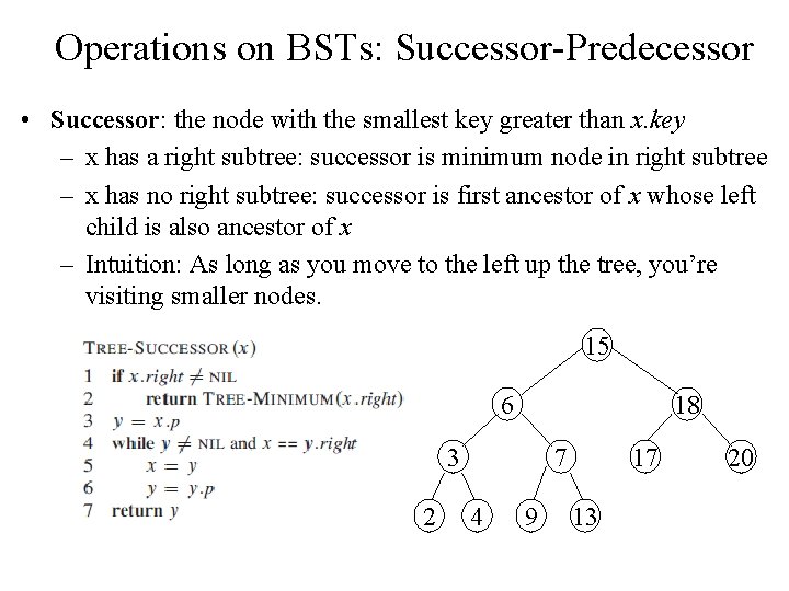
Operations on BSTs: Successor-Predecessor • Successor: the node with the smallest key greater than x. key – x has a right subtree: successor is minimum node in right subtree – x has no right subtree: successor is first ancestor of x whose left child is also ancestor of x – Intuition: As long as you move to the left up the tree, you’re visiting smaller nodes. 15 6 18 3 2 7 4 9 17 13 20

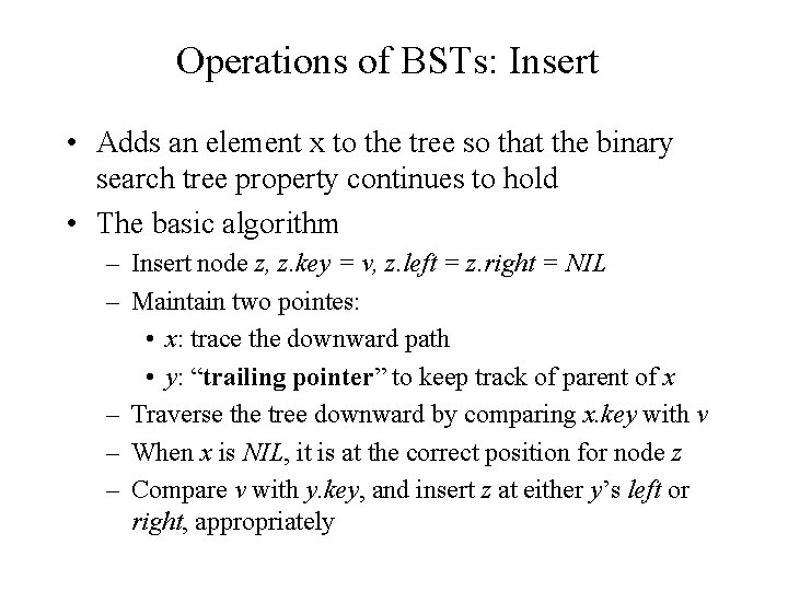
Operations of BSTs: Insert • Adds an element x to the tree so that the binary search tree property continues to hold • The basic algorithm – Insert node z, z. key = v, z. left = z. right = NIL – Maintain two pointes: • x: trace the downward path • y: “trailing pointer” to keep track of parent of x – Traverse the tree downward by comparing x. key with v – When x is NIL, it is at the correct position for node z – Compare v with y. key, and insert z at either y’s left or right, appropriately

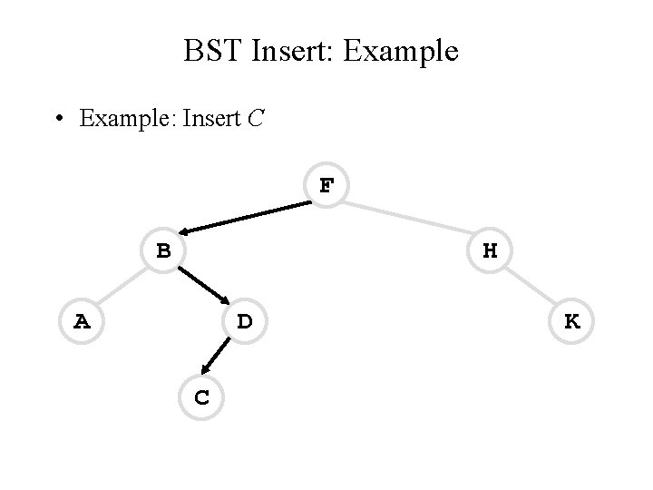
BST Insert: Example • Example: Insert C F B H A D C K

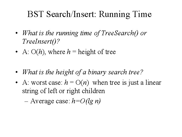
BST Search/Insert: Running Time • What is the running time of Tree. Search() or Tree. Insert()? • A: O(h), where h = height of tree • What is the height of a binary search tree? • A: worst case: h = O(n) when tree is just a linear string of left or right children – Average case: h=O(lg n)

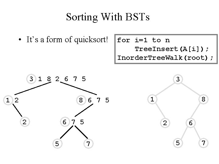
Sorting With BSTs • It’s a form of quicksort! for i=1 to n Tree. Insert(A[i]); Inorder. Tree. Walk(root); 3 1 8 2 6 7 5 1 2 3 8 6 7 5 2 6 7 5 5 1 8 2 7 6 5 7

Sorting with BSTs • Which do you think is better, quicksort or BSTSort? Why? • A: quicksort – Sorts in place – Doesn’t need to build data structure

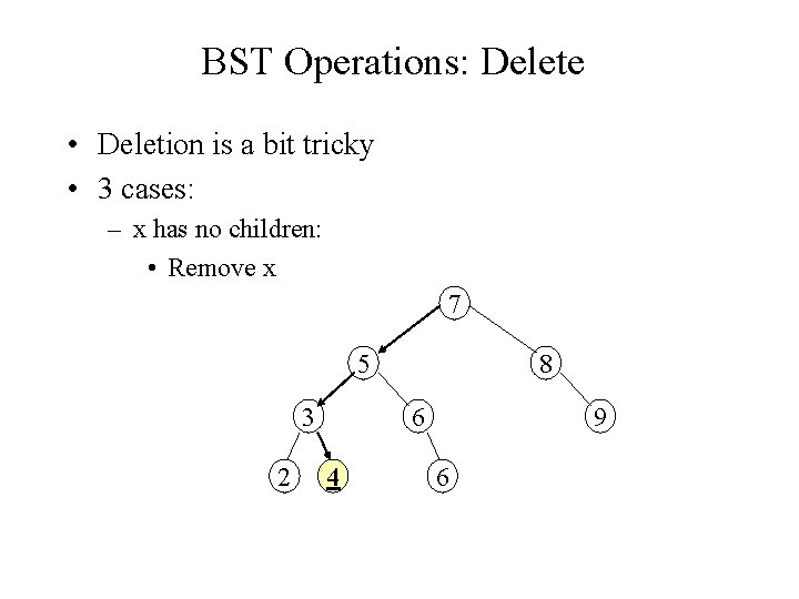
BST Operations: Delete • Deletion is a bit tricky • 3 cases: – x has no children: • Remove x 7 5 3 2 8 6 4 9 6

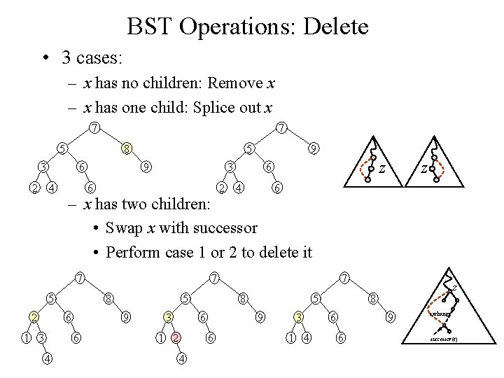
BST Operations: Delete • 3 cases: – x has no children: Remove x – x has one child: Splice out x 7 7 5 8 3 2 6 4 5 9 9 3 6 2 z 6 4 z 6 – x has two children: • Swap x with successor • Perform case 1 or 2 to delete it 7 5 2 8 6 1 3 5 9 6 4 7 3 8 6 1 2 5 9 6 4 7 3 1 4 z 8 6 9 6 exchange successor(z)

BST Operations: Delete • Why will case 2 always go to case 0 or case 1? • A: because when x has 2 children, its successor is the minimum in its right subtree, and that successor has no left child (hence 0 or 1 child). • Could we swap x with predecessor instead of successor? • A: yes. • Would it be a good idea? • A: might be good to alternate to avoid creating unbalanced tree.