CS 598 VISUAL INFORMATION RETRIEVAL Lecture III Image

CS 598: VISUAL INFORMATION RETRIEVAL Lecture III: Image Representation: Invariant Local Image Descriptors

RECAP OF LECTURE II Color, texture, descriptors � Color histogram � Color correlogram � LBP descriptors � Histogram of oriented gradient � Spatial pyramid matching Distance & Similarity measure � Lp distances � Chi-Square distances � KL distances � EMD distances � Histogram intersection

LECTURE III: PART I Local Feature Detector

OUTLINE Blob detection � Brief of Gaussian filter � Scale selection � Lapacian of Gaussian (Lo. G) detector � Difference of Gaussian (Do. G) detector � Affine co-variant region

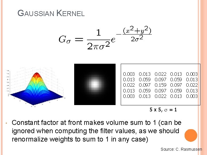
GAUSSIAN KERNEL 0. 003 0. 013 0. 022 0. 013 0. 003 0. 013 0. 059 0. 097 0. 059 0. 013 0. 022 0. 097 0. 159 0. 097 0. 022 0. 013 0. 059 0. 097 0. 059 0. 013 0. 003 0. 013 0. 022 0. 013 0. 003 5 x 5, = 1 • Constant factor at front makes volume sum to 1 (can be ignored when computing the filter values, as we should renormalize weights to sum to 1 in any case) Source: C. Rasmussen

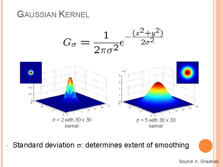
GAUSSIAN KERNEL σ = 2 with 30 x 30 kernel • σ = 5 with 30 x 30 kernel Standard deviation : determines extent of smoothing Source: K. Grauman

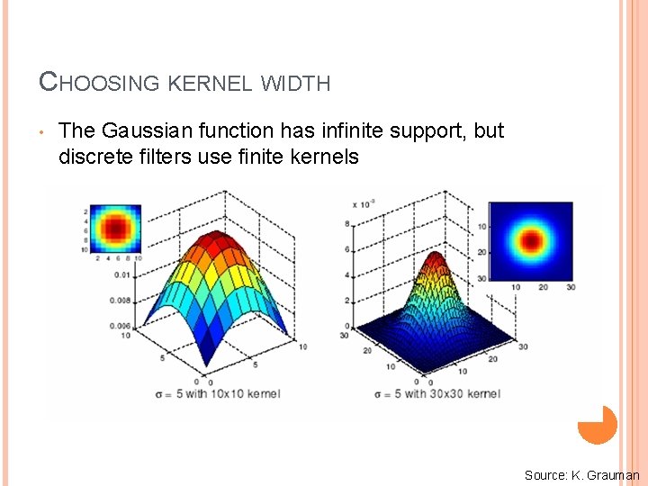
CHOOSING KERNEL WIDTH • The Gaussian function has infinite support, but discrete filters use finite kernels Source: K. Grauman

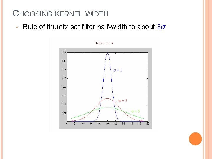
CHOOSING KERNEL WIDTH • Rule of thumb: set filter half-width to about 3σ

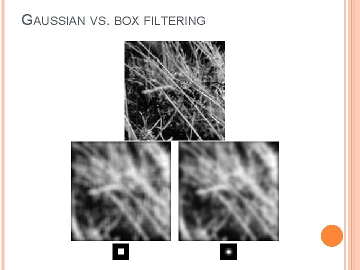
GAUSSIAN VS. BOX FILTERING

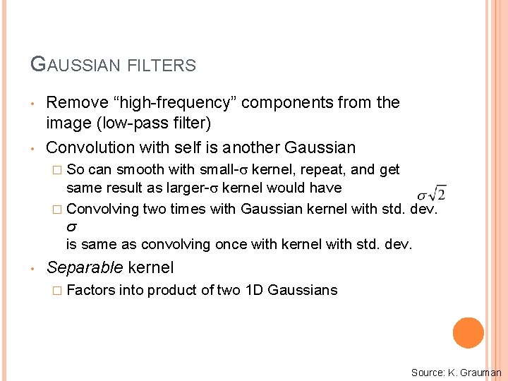
GAUSSIAN FILTERS • • Remove “high-frequency” components from the image (low-pass filter) Convolution with self is another Gaussian � So can smooth with small- kernel, repeat, and get same result as larger- kernel would have � Convolving two times with Gaussian kernel with std. dev. σ is same as convolving once with kernel with std. dev. • Separable kernel � Factors into product of two 1 D Gaussians Source: K. Grauman

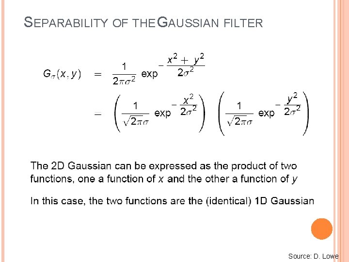
SEPARABILITY OF THE GAUSSIAN FILTER Source: D. Lowe

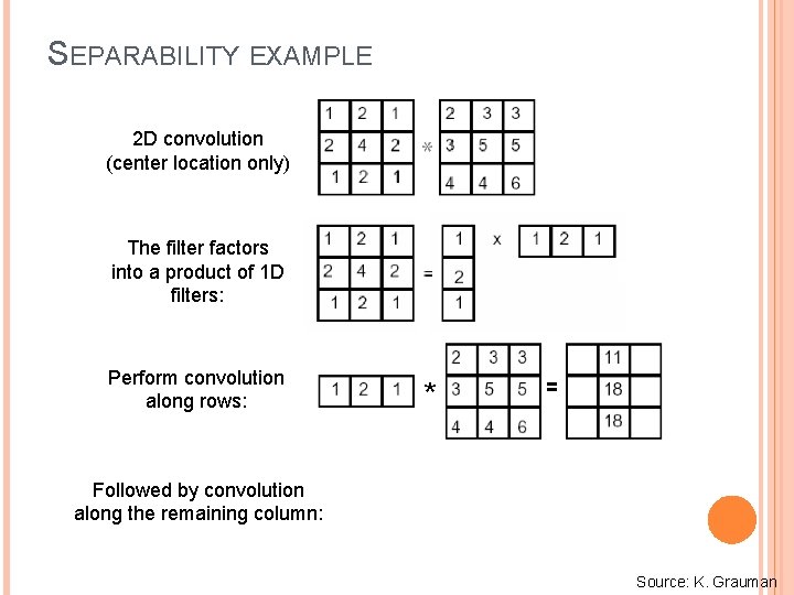
SEPARABILITY EXAMPLE 2 D convolution (center location only) The filter factors into a product of 1 D filters: Perform convolution along rows: Followed by convolution along the remaining column: * = Source: K. Grauman

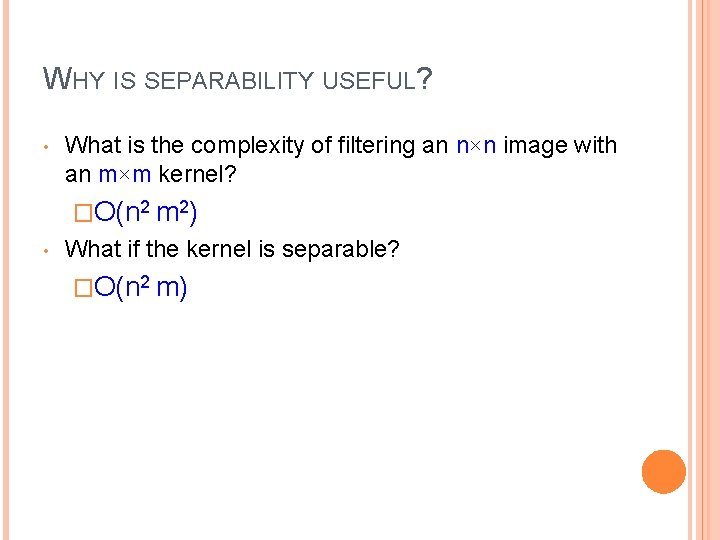
WHY IS SEPARABILITY USEFUL? • What is the complexity of filtering an n×n image with an m×m kernel? �O(n 2 m 2) • What if the kernel is separable? �O(n 2 m)

OUTLINE Blob detection � Brief of Gaussian filter � Scale selection � Lapacian of Gaussian (Lo. G) detector � Difference of Gaussian (Do. G) detector � Affine co-variant region

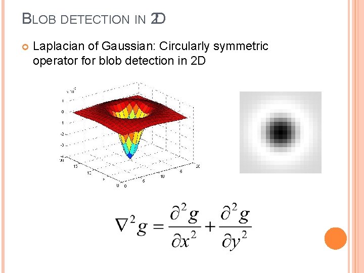
BLOB DETECTION IN 2 D Laplacian of Gaussian: Circularly symmetric operator for blob detection in 2 D

BLOB DETECTION IN 2 D Laplacian of Gaussian: Circularly symmetric operator for blob detection in 2 D Scale-normalized:

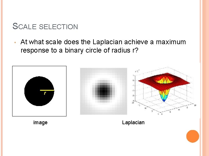
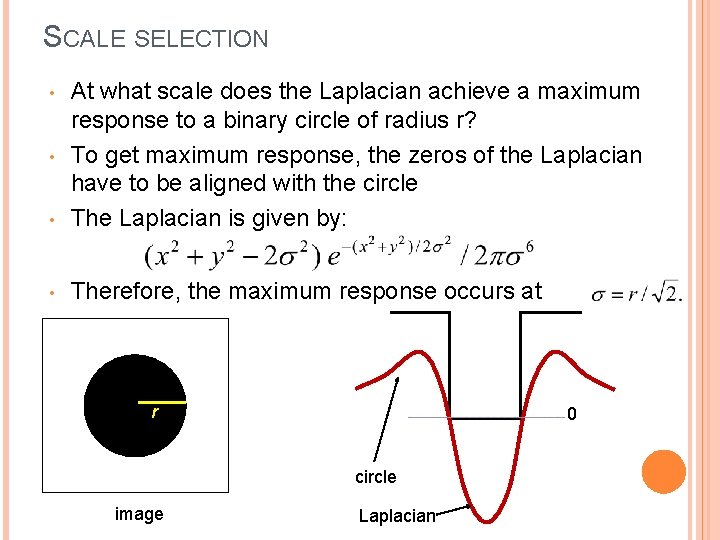
SCALE SELECTION • At what scale does the Laplacian achieve a maximum response to a binary circle of radius r? r image Laplacian

SCALE SELECTION • At what scale does the Laplacian achieve a maximum response to a binary circle of radius r? To get maximum response, the zeros of the Laplacian have to be aligned with the circle The Laplacian is given by: • Therefore, the maximum response occurs at • • r 0 circle image Laplacian

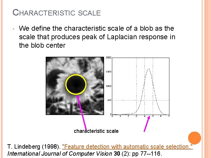
CHARACTERISTIC SCALE • We define the characteristic scale of a blob as the scale that produces peak of Laplacian response in the blob center characteristic scale T. Lindeberg (1998). "Feature detection with automatic scale selection. " International Journal of Computer Vision 30 (2): pp 77 --116.

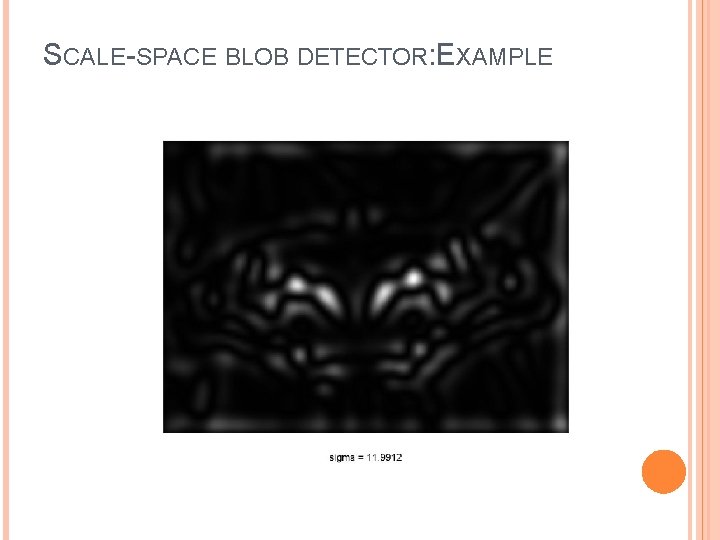
SCALE-SPACE BLOB DETECTOR 1. Convolve image with scale-normalized Laplacian at several scales

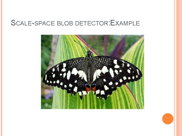
SCALE-SPACE BLOB DETECTOR: EXAMPLE

SCALE-SPACE BLOB DETECTOR: EXAMPLE

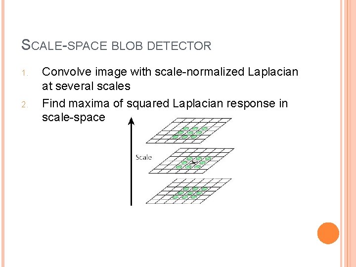
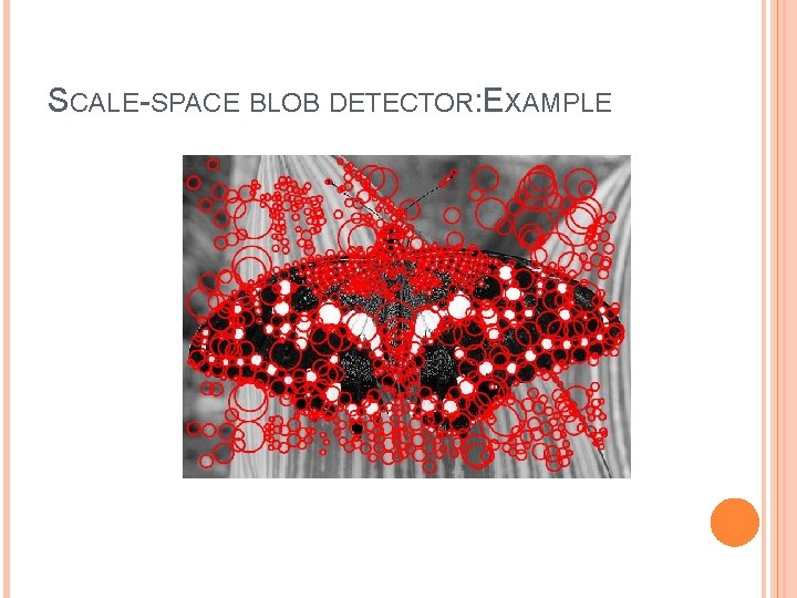
SCALE-SPACE BLOB DETECTOR 1. 2. Convolve image with scale-normalized Laplacian at several scales Find maxima of squared Laplacian response in scale-space

SCALE-SPACE BLOB DETECTOR: EXAMPLE

OUTLINE Blob detection � Brief of Gaussian filter � Scale selection � Lapacian of Gaussian (Lo. G) detector � Difference of Gaussian (Do. G) detector � Affine co-variant region

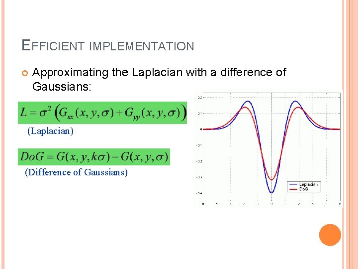
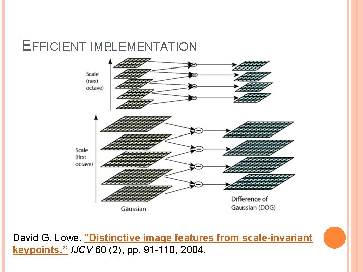
EFFICIENT IMPLEMENTATION Approximating the Laplacian with a difference of Gaussians: (Laplacian) (Difference of Gaussians)

EFFICIENT IMPLEMENTATION David G. Lowe. "Distinctive image features from scale-invariant keypoints. ” IJCV 60 (2), pp. 91 -110, 2004.

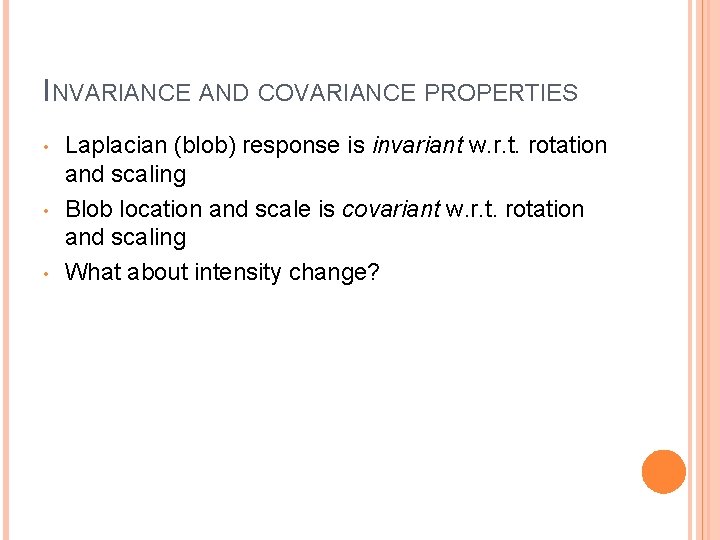
INVARIANCE AND COVARIANCE PROPERTIES • • • Laplacian (blob) response is invariant w. r. t. rotation and scaling Blob location and scale is covariant w. r. t. rotation and scaling What about intensity change?

OUTLINE Blob detection � Brief of Gaussian filter � Scale selection � Lapacian of Gaussian (Lo. G) detector � Difference of Gaussian (Do. G) detector � Affine co-variant region

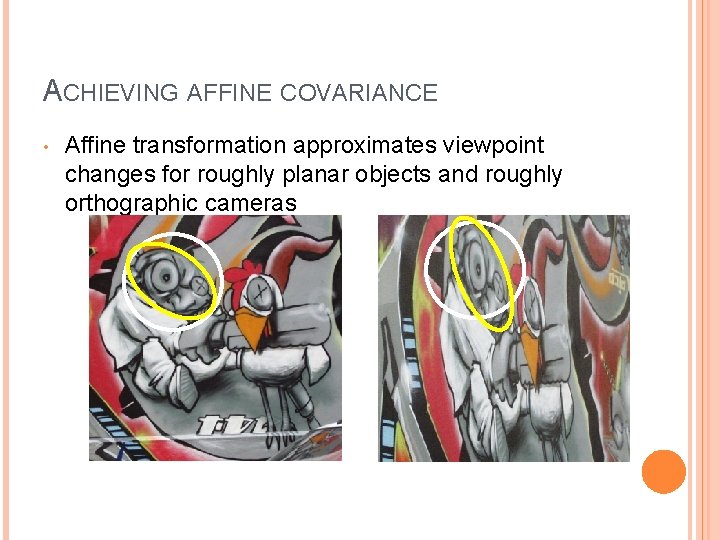
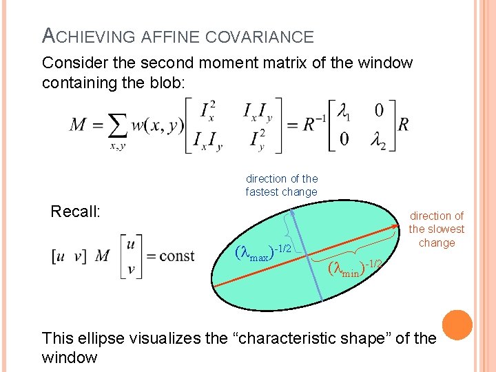
ACHIEVING AFFINE COVARIANCE • Affine transformation approximates viewpoint changes for roughly planar objects and roughly orthographic cameras

ACHIEVING AFFINE COVARIANCE Consider the second moment matrix of the window containing the blob: direction of the fastest change Recall: ( max)-1/2 direction of the slowest change ( min)-1/2 This ellipse visualizes the “characteristic shape” of the window

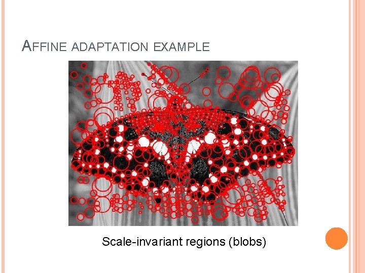
AFFINE ADAPTATION EXAMPLE Scale-invariant regions (blobs)

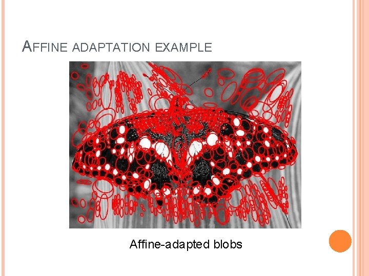
AFFINE ADAPTATION EXAMPLE Affine-adapted blobs

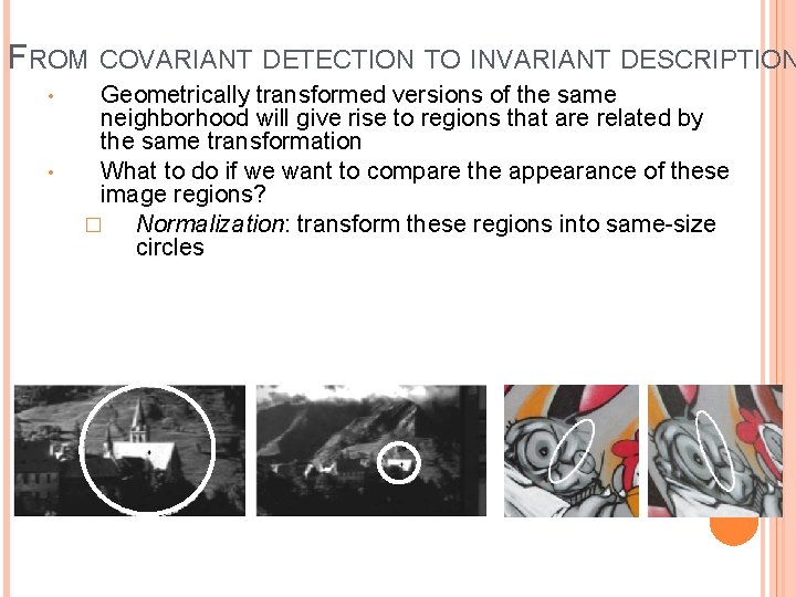
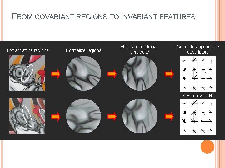
FROM COVARIANT DETECTION TO INVARIANT DESCRIPTION • • Geometrically transformed versions of the same neighborhood will give rise to regions that are related by the same transformation What to do if we want to compare the appearance of these image regions? � Normalization: transform these regions into same-size circles

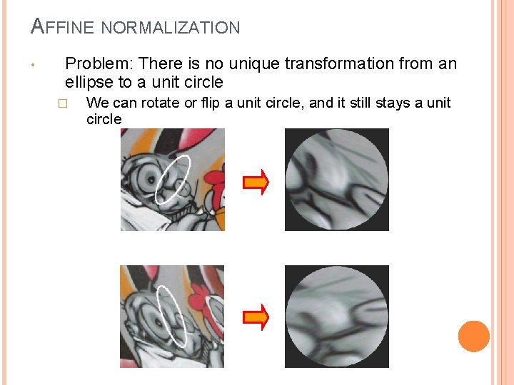
AFFINE NORMALIZATION • Problem: There is no unique transformation from an ellipse to a unit circle � We can rotate or flip a unit circle, and it still stays a unit circle

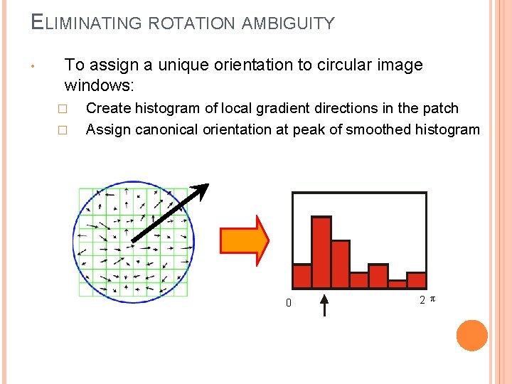
ELIMINATING ROTATION AMBIGUITY • To assign a unique orientation to circular image windows: � � Create histogram of local gradient directions in the patch Assign canonical orientation at peak of smoothed histogram 0 2 p

FROM COVARIANT REGIONS TO INVARIANT FEATURES Extract affine regions Normalize regions Eliminate rotational ambiguity Compute appearance descriptors SIFT (Lowe ’ 04)

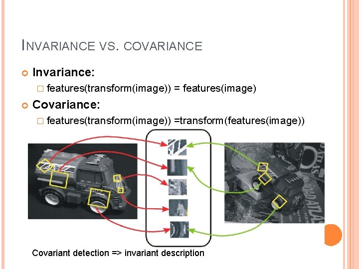
INVARIANCE VS. COVARIANCE Invariance: � features(transform(image)) = features(image) Covariance: � features(transform(image)) =transform(features(image)) Covariant detection => invariant description

David G. Lowe, “Distinctive Image Features from Scale-Invariant Keypoints”, International Journal of Computer Vision, Vol. 60, No. 2, pp. 91 -110 • 6291 as of 02/28/2010; 22481 as of 02/03/2014 • Our goal is to design the best local image descriptors in the world. LECTURE III: PART I Learning Local Feature Descriptor

Panoramic stitching [Brown et al. CVPR 05] Real-world. Face recognition [Wright & Hua CVPR 09] [Hua & Akbarzadeh ICCV 09] Image databases [Mikolajczyk & Schmid ICCV 01] Courtesy of Seitz & Szeliski Object or location recognition [Nister & Stewenius CVPR 06] Robot navigation [Deans et al. AC 05] 3 D reconstruction [Snavely et al. SIGGRAPH 06]

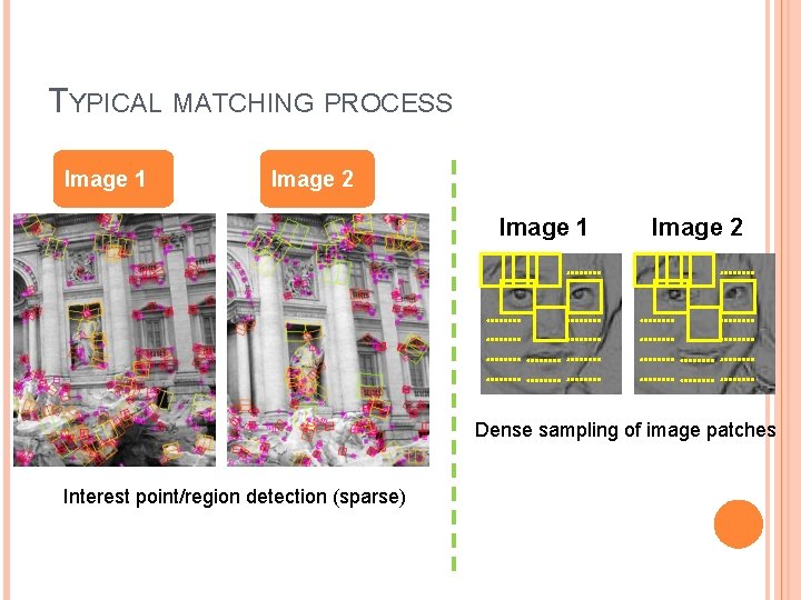
TYPICAL MATCHING PROCESS Image 1 Image 2 Dense sampling of image patches Interest point/region detection (sparse)

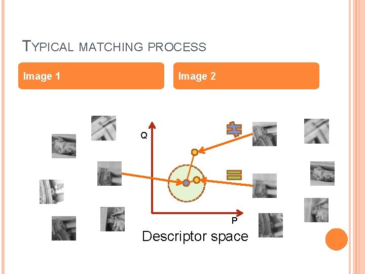
TYPICAL MATCHING PROCESS Image 1 Image 2 Q P Descriptor space

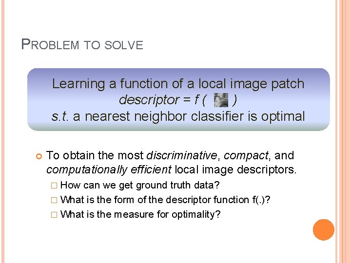
PROBLEM TO SOLVE Learning a function of a local image patch descriptor = f ( ) s. t. a nearest neighbor classifier is optimal To obtain the most discriminative, compact, and computationally efficient local image descriptors. � How can we get ground truth data? � What is the form of the descriptor function f(. )? � What is the measure for optimality?

HOW CAN WE GET GROUND TRUTH DATA?

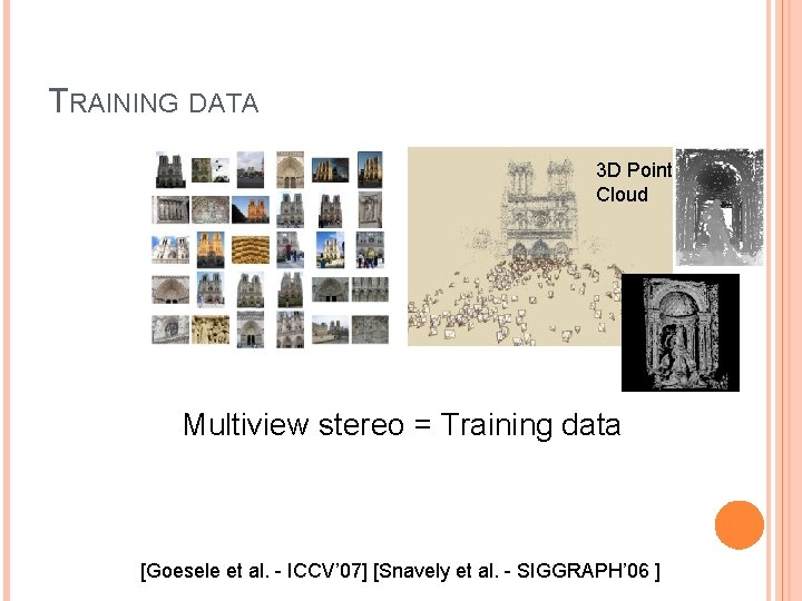
TRAINING DATA 3 D Point Cloud Multiview stereo = Training data [Goesele et al. - ICCV’ 07] [Snavely et al. - SIGGRAPH’ 06 ]

TRAINING DATA 3 D Point Cloud [Goesele et al. - ICCV’ 07] [Snavely et al. - SIGGRAPH’ 06 ]

TRAINING DATA 3 D Point Cloud [Goesele et al. - ICCV’ 07] [Snavely et al. - SIGGRAPH’ 06 ]

TRAINING DATA 3 D Point Cloud [Goesele et al. - ICCV’ 07] [Snavely et al. - SIGGRAPH’ 06 ]

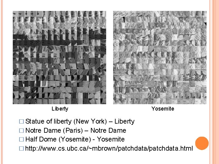
Liberty Yosemite � Statue of liberty (New York) – Liberty � Notre Dame (Paris) – Notre Dame � Half Dome (Yosemite) - Yosemite � http: //www. cs. ubc. ca/~mbrown/patchdata. html

WHAT IS THE FORM OF THE DESCRIPTOR FUNCTION?

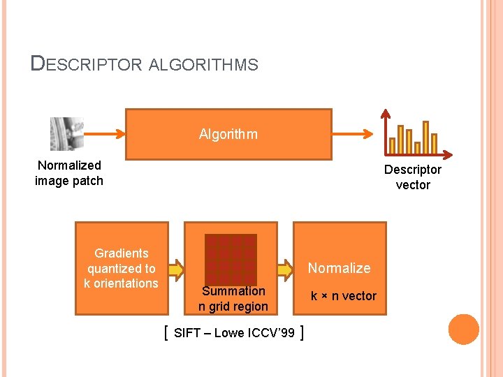
DESCRIPTOR ALGORITHMS Algorithm Normalized image patch Gradients quantized to k orientations Descriptor vector Normalize Summation n grid region [ SIFT – Lowe ICCV’ 99 ] k × n vector

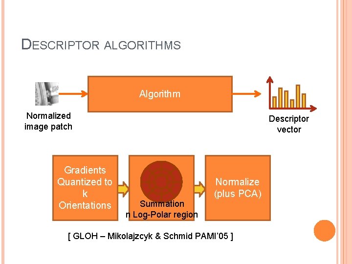
DESCRIPTOR ALGORITHMS Algorithm Normalized image patch Gradients Quantized to k Orientations Descriptor vector Summation n Log-Polar region Normalize (plus PCA) [ GLOH – Mikolajzcyk & Schmid PAMI’ 05 ]

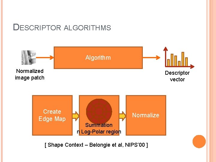
DESCRIPTOR ALGORITHMS Algorithm Normalized image patch Descriptor vector Create Edge Map Normalize Summation n Log-Polar region [ Shape Context – Belongie et al, NIPS’ 00 ]

DESCRIPTOR ALGORITHMS Algorithm Normalized image patch Grey value quantized into k bins Descriptor vector Normalize Summation n circular region [ Spin Image – Lazebnik et al, CVPR’ 03 ]

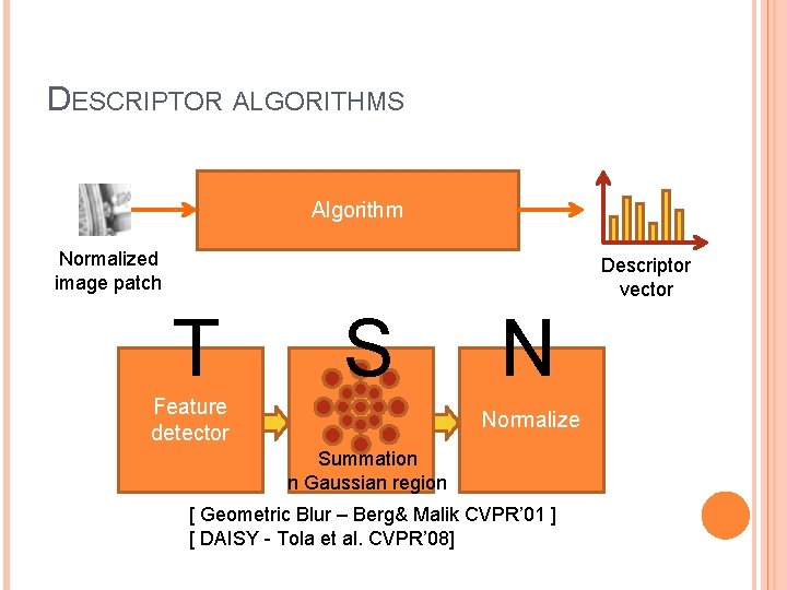
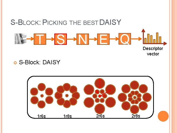
DESCRIPTOR ALGORITHMS Algorithm Normalized image patch Descriptor vector T S Feature detector N Normalize Summation n Gaussian region [ Geometric Blur – Berg& Malik CVPR’ 01 ] [ DAISY - Tola et al. CVPR’ 08]

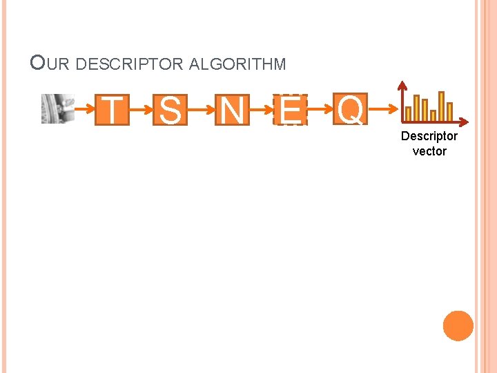
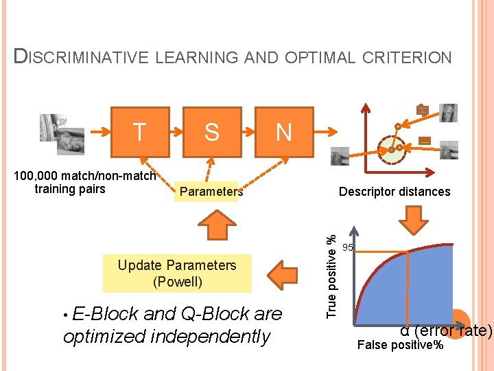
OUR DESCRIPTOR ALGORITHM T S N E Q Descriptor vector

S-BLOCK: PICKING THE BEST DAISY T S N E Q Descriptor vector S-Block: DAISY 1 r 6 s 1 r 8 s 2 r 6 s 2 r 8 s

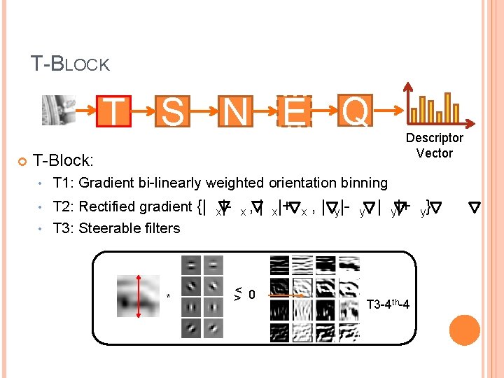
T-BLOCK T S N E Q T-Block: • Descriptor Vector T 1: Gradient bi-linearly weighted orientation binning T 2: Rectified gradient {| x|- x , | x|+ x , | y|- y , | y|+ y} • T 3: Steerable filters • * < > 0 T 3 -4 th-4

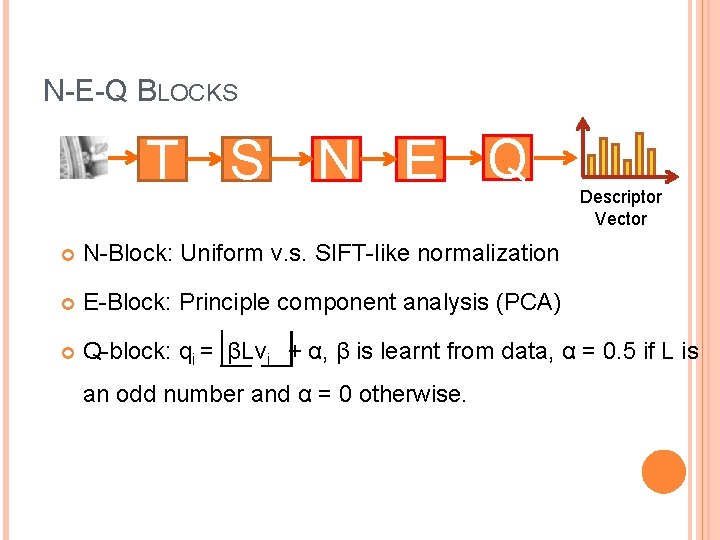
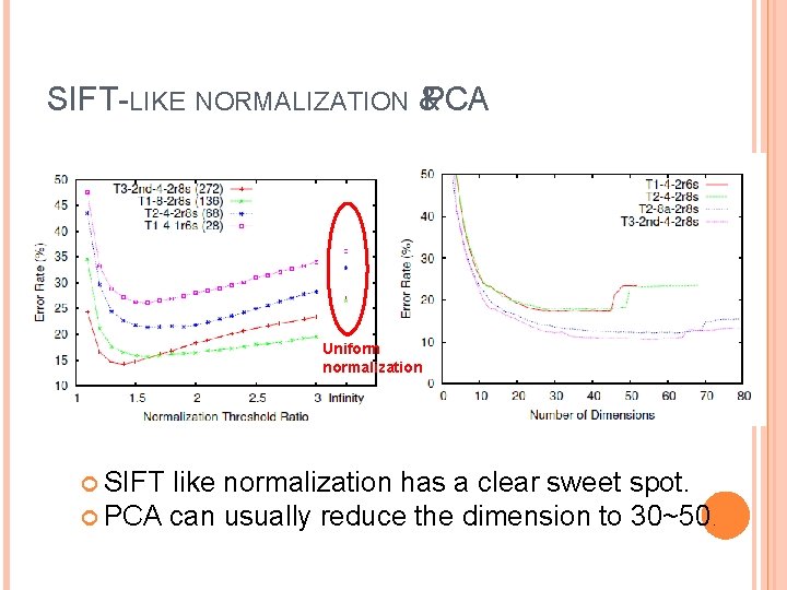
N-E-Q BLOCKS T S N E Q Descriptor Vector N-Block: Uniform v. s. SIFT-like normalization E-Block: Principle component analysis (PCA) Q-block: qi = βLvi + α, β is learnt from data, α = 0. 5 if L is an odd number and α = 0 otherwise.

WHAT IS THE OPTIMAL CRITERION?

DISCRIMINATIVE LEARNING AND OPTIMAL CRITERION 100, 000 match/non-match training pairs S N Update Parameters (Powell) • E-Block Descriptor distances Parameters and Q-Block are optimized independently True positive % T 95 α (error rate) False positive%

SIFT-LIKE NORMALIZATION & PCA Uniform normalization SIFT like normalization has a clear sweet spot. PCA can usually reduce the dimension to 30~50.

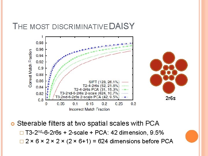
THE MOST DISCRIMINATIVE DAISY 2 r 6 s Steerable filters at two spatial scales with PCA � T 3 -2 nd-6 -2 r 6 s + 2 -scale + PCA: 42 dimension, 9. 5% � 2 × 6 × 2 × (2 × 6+1) = 624 dimensions before PCA

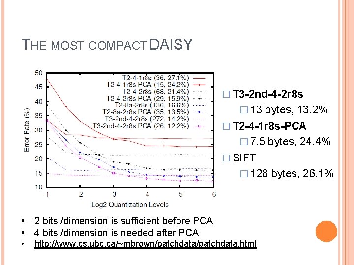
THE MOST COMPACT DAISY � T 3 -2 nd-4 -2 r 8 s � 13 bytes, 13. 2% � T 2 -4 -1 r 8 s-PCA � 7. 5 bytes, 24. 4% � SIFT � 128 bytes, 26. 1% • 2 bits /dimension is sufficient before PCA • 4 bits /dimension is needed after PCA • http: //www. cs. ubc. ca/~mbrown/patchdata. html

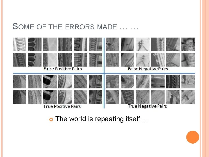
SOME OF THE ERRORS MADE … … The world is repeating itself….

SUMMARY Blob detection � Brief of Gaussian filter � Scale selection � Lapacian of Gaussian (Lo. G) detector � Difference of Gaussian (Do. G) detector � Affine co-variant region Learning local descriptors � How can we get ground-truth data? � What is the form of the descriptor function? � What is the optimal criterion? � How do we optimize it?