CS 580 Monte Carlo Ray Tracing Part I

CS 580: Monte Carlo Ray Tracing: Part I Sung-Eui Yoon (윤성의) Course URL: http: //sglab. kaist. ac. kr/~sungeui/GCG

Class Objectives ● Understand a basic structure of Monte Carlo ray tracing ● Russian roulette for its termination ● Stratified sampling ● Quasi-Monte Carlo ray tracing 2

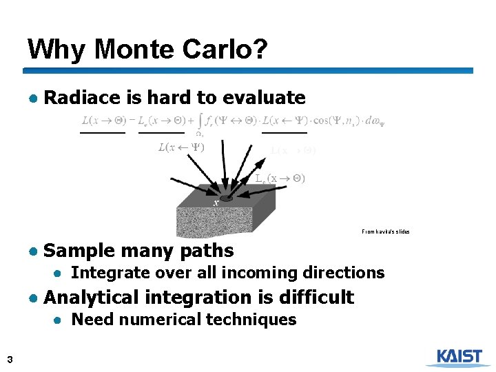
Why Monte Carlo? ● Radiace is hard to evaluate From kavita’s slides ● Sample many paths ● Integrate over all incoming directions ● Analytical integration is difficult ● Need numerical techniques 3

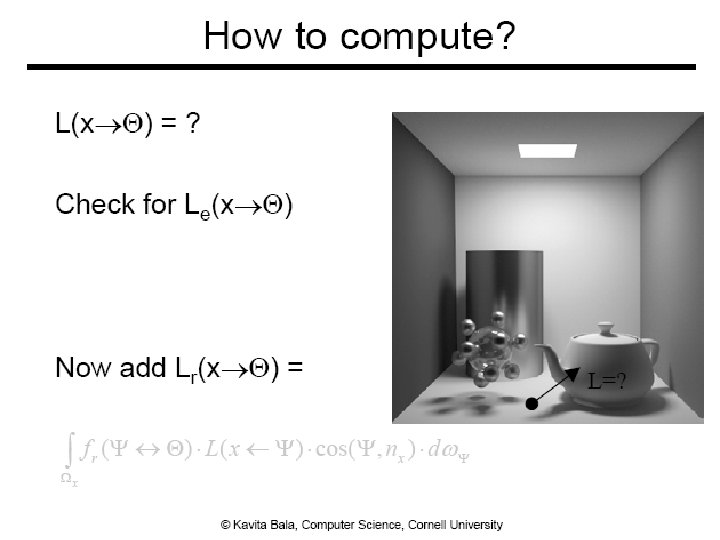
Rendering Equation 4

5

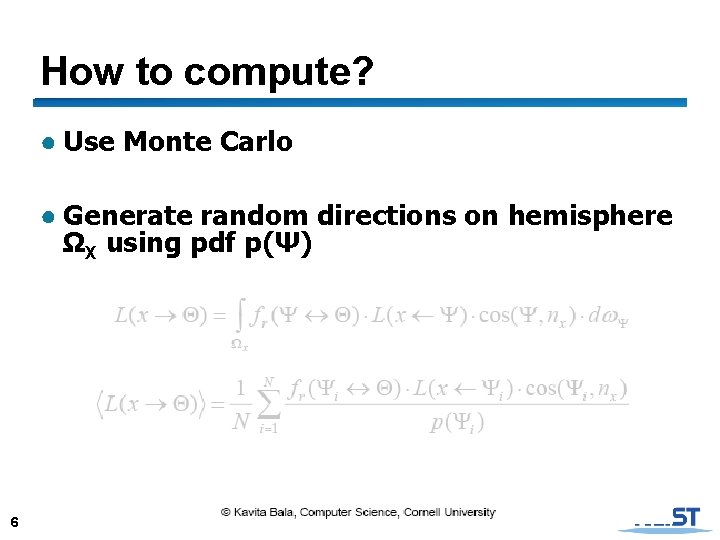
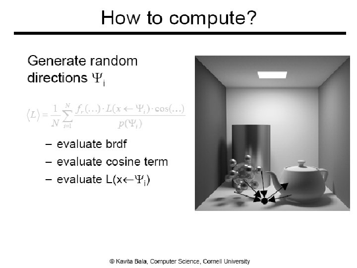
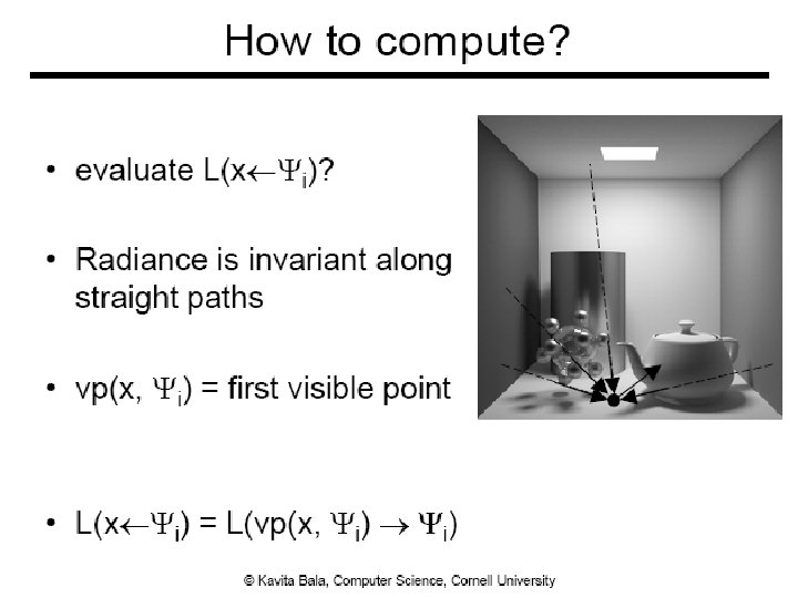
How to compute? ● Use Monte Carlo ● Generate random directions on hemisphere ΩX using pdf p(Ψ) 6

7

8

9

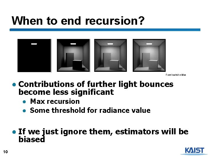
When to end recursion? From kavita’s slides ● Contributions of further light bounces become less significant ● Max recursion ● Some threshold for radiance value ● If we just ignore them, estimators will be biased 10

11

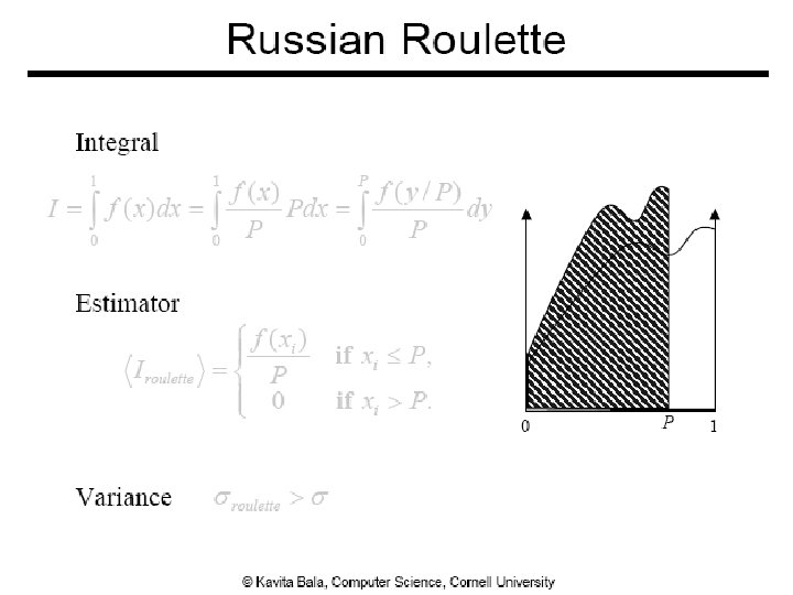
Russian Roulette ● Pick absorption probability, α = 1 -P ● Recursion is terminated ● 1 - α = P is commonly to be equal to the reflectance of the material of the surface ● Darker surface absorbs more paths 12

Algorithm so far ● Shoot primary rays through each pixel ● Shoot indirect rays, sampled over hemisphere ● Terminate recursion using Russian Roulette 13

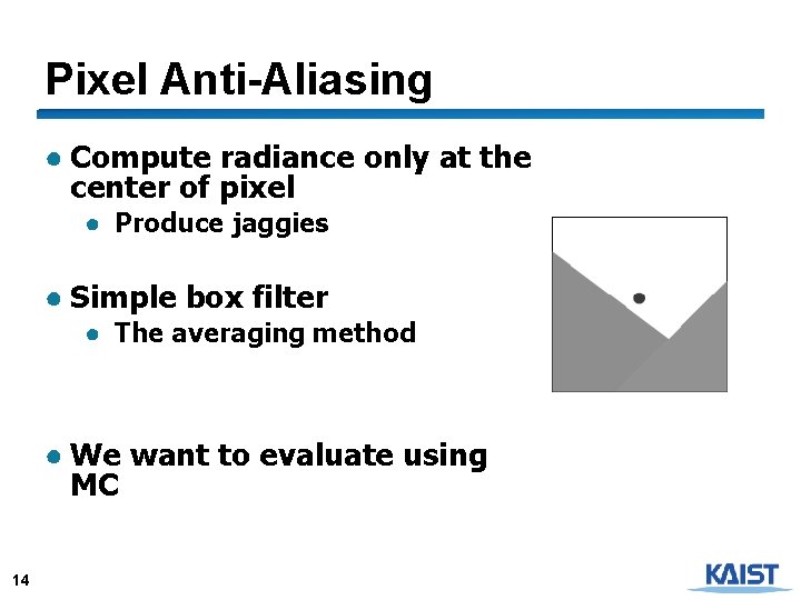
Pixel Anti-Aliasing ● Compute radiance only at the center of pixel ● Produce jaggies ● Simple box filter ● The averaging method ● We want to evaluate using MC 14

Stochastic Ray Tracing ● Parameters ● Num. of starting ray per pixel ● Num. of random rays for each surface point (branching factor) ● Path tracing ● Branching factor = 1 15

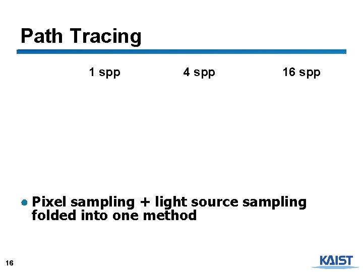
Path Tracing 1 spp 4 spp 16 spp ● Pixel sampling + light source sampling folded into one method 16

Algorithm so far ● Shoot primary rays through each pixel ● Shoot indirect rays, sampled over hemisphere ● Path tracing shoots only 1 indirect ray ● Terminate recursion using Russian Roulette 17

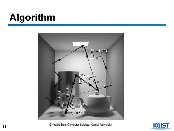
Algorithm 18

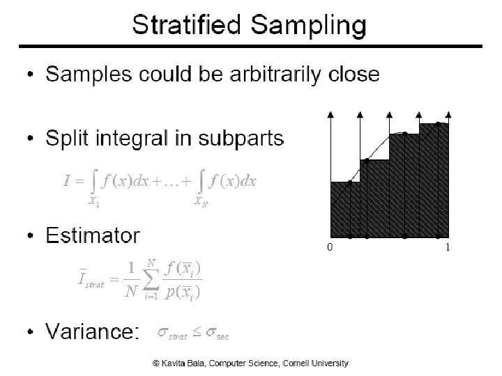
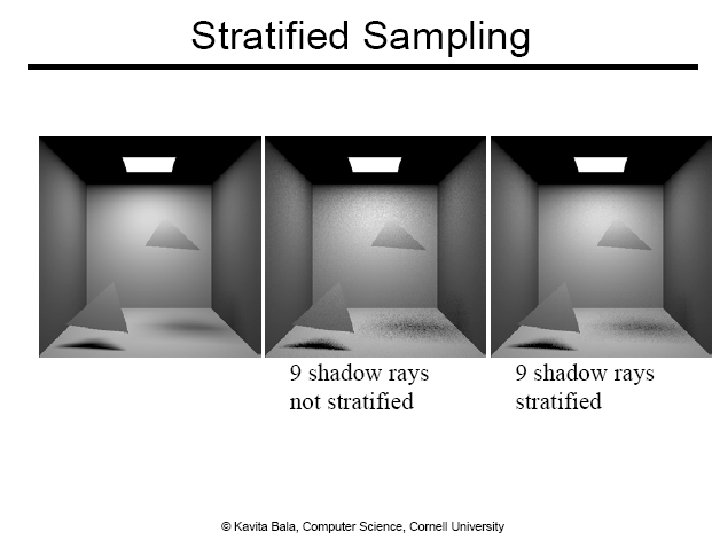
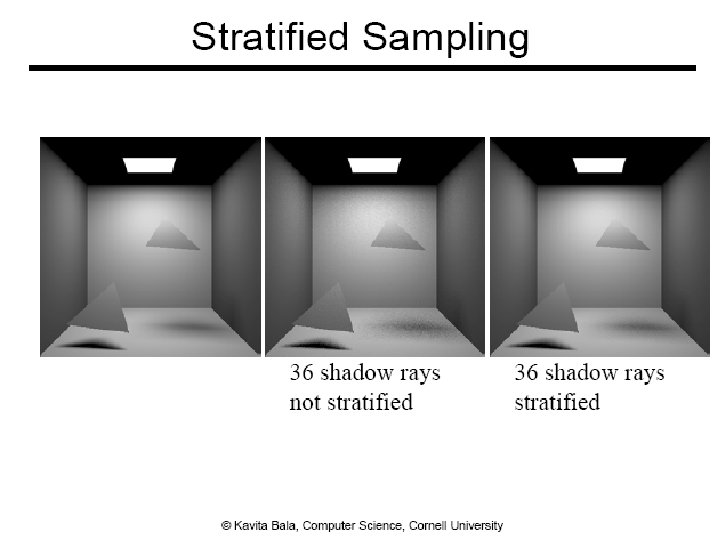
Performance ● Want better quality with smaller # of samples ● Fewer samples/better performance ● Stratified sampling ● Quasi Monte Carlo: well-distributed samples ● Faster convergence ● Importance sampling 19

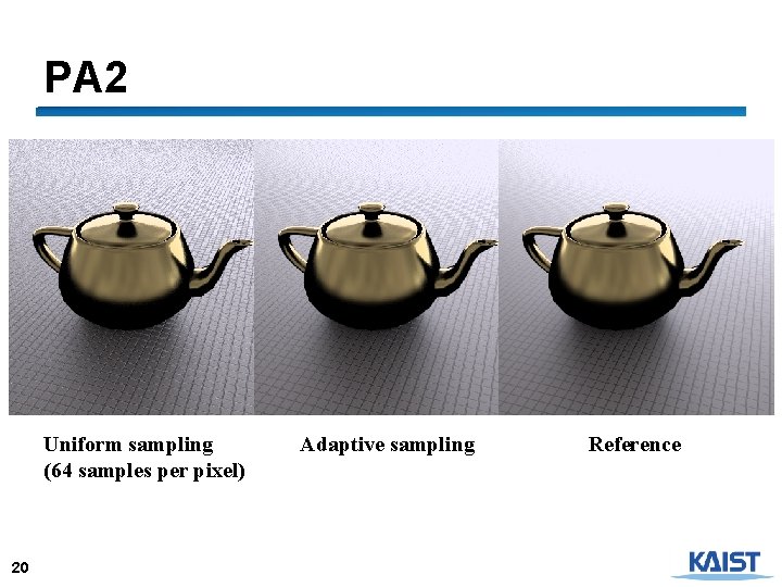
PA 2 Uniform sampling (64 samples per pixel) 20 Adaptive sampling Reference

21

22

23

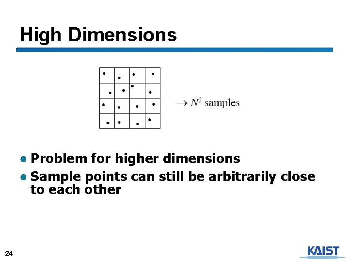
High Dimensions ● Problem for higher dimensions ● Sample points can still be arbitrarily close to each other 24

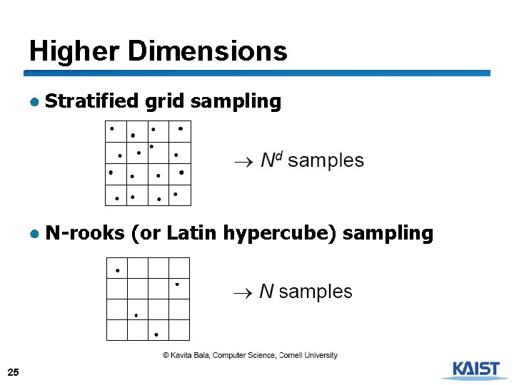
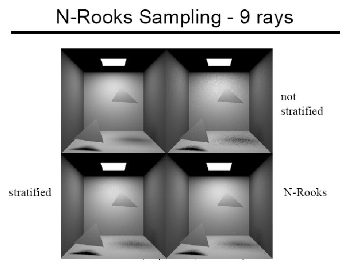
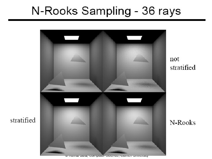
Higher Dimensions ● Stratified grid sampling ● N-rooks (or Latin hypercube) sampling 25

26

27

Sobol Sequence ● Attempt to have one sample in different elementary intervals All elementary intervals having the volume of 1/16 28 Jittered Sobol N-Rooks Images are from Kollig and Keller’s EG 2002

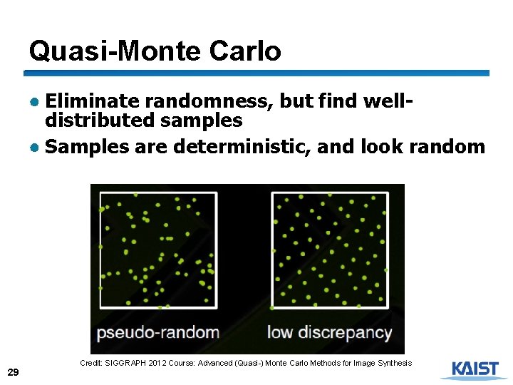
Quasi-Monte Carlo ● Eliminate randomness, but find welldistributed samples ● Samples are deterministic, and look random 29 Credit: SIGGRAPH 2012 Course: Advanced (Quasi-) Monte Carlo Methods for Image Synthesis

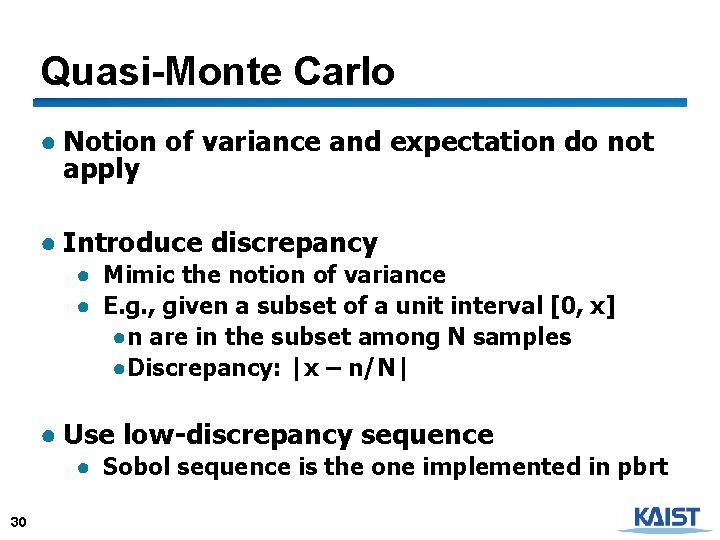
Quasi-Monte Carlo ● Notion of variance and expectation do not apply ● Introduce discrepancy ● Mimic the notion of variance ● E. g. , given a subset of a unit interval [0, x] ●n are in the subset among N samples ●Discrepancy: |x – n/N| ● Use low-discrepancy sequence ● Sobol sequence is the one implemented in pbrt 30

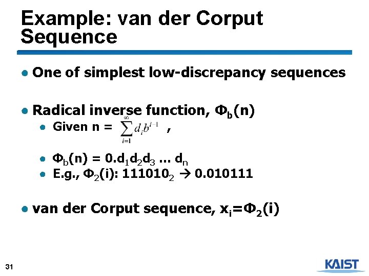
Example: van der Corput Sequence ● One of simplest low-discrepancy sequences ● Radical inverse function, Φb(n) ● Given n = , ● Φb(n) = 0. d 1 d 2 d 3 … dn ● E. g. , Φ 2(i): 1110102 0. 010111 ● van der Corput sequence, xi=Φ 2(i) 31

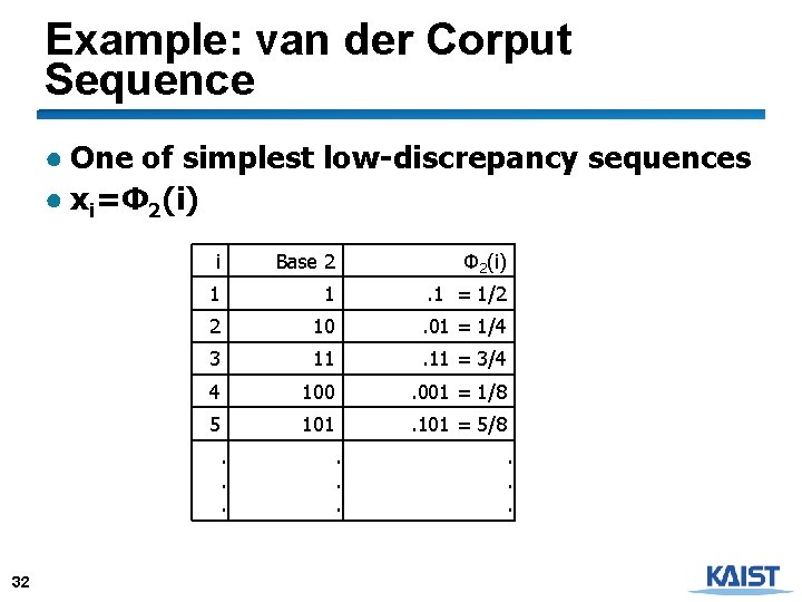
Example: van der Corput Sequence ● One of simplest low-discrepancy sequences ● xi=Φ 2(i) i Base 2 Φ 2(i) 1 1 . 1 = 1/2 2 10 . 01 = 1/4 3 11 = 3/4 4 100 . 001 = 1/8 5 101 = 5/8 . . . 32 . . .

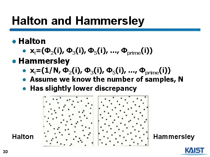
Halton and Hammersley ● Halton ● xi=(Φ 2(i), Φ 3(i), Φ 5(i), …, Φprime(i)) ● Hammersley ● xi=(1/N, Φ 2(i), Φ 3(i), Φ 5(i), …, Φprime(i)) ● Assume we know the number of samples, N ● Has slightly lower discrepancy Halton 33 Hammersley

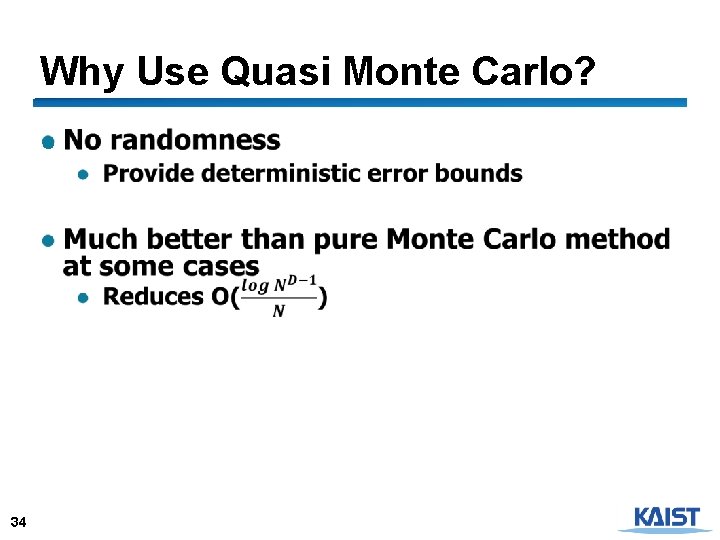
Why Use Quasi Monte Carlo? ● 34

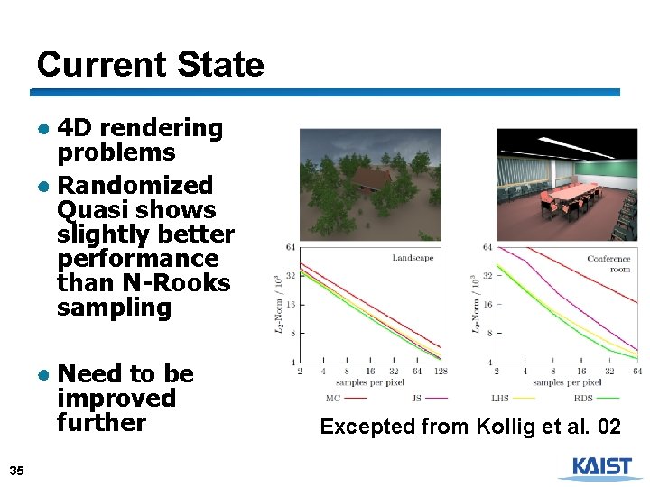
Current State ● 4 D rendering problems ● Randomized Quasi shows slightly better performance than N-Rooks sampling ● Need to be improved further 35 Excepted from Kollig et al. 02

Performance and Error ● Want better quality with smaller number of samples ● Fewer samples better performance ● Stratified sampling ● Quasi Monte Carlo: well-distributed samples ● Faster convergence ● Importance sampling: next-event estimation 36

Class Objectives were: ● Understand a basic structure of Monte Carlo ray tracing ● Russian roulette for its termination ● Stratified sampling ● Quasi-Monte Carlo ray tracing 37

Homework ● Go over the next lecture slides before the class ● Watch 2 SIGGRAPH videos and submit your summaries every Tue. class ● Just one paragraph for each summary Example: Title: XXXX Abstract: this video is about accelerating the performance of ray tracing. To achieve its goal, they design a new technique for reordering rays, since by doing so, they can improve the ray coherence and thus improve the overall performance. 38

Any Questions? ● Come up with one question on what we have discussed in the class and submit at the end of the class ● 1 for already answered questions ● 2 for typical questions ● 3 for questions with thoughts ● Submit questions at least four times before the mid-term exam ● Multiple questions for the class is counted as only a single time 39

Next Time ● Importance sampling for MC ray tracing 40

Figures 41