CS 559 Computer Graphics Lecture 24 Shape Modeling

CS 559: Computer Graphics Lecture 24: Shape Modeling Li Zhang Spring 2010

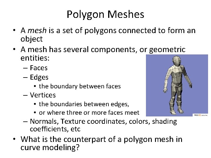
Polygon Meshes • A mesh is a set of polygons connected to form an object • A mesh has several components, or geometric entities: – Faces – Edges • the boundary between faces – Vertices • the boundaries between edges, • or where three or more faces meet – Normals, Texture coordinates, colors, shading coefficients, etc • What is the counterpart of a polygon mesh in curve modeling?

Open. GL and Vertex Indirection struct Vertex { float coords[3]; } struct Triangle { GLuint verts[3]; } struct Mesh { struct Vertex vertices[m]; struct Triangle triangles[n]; } gl. Enable. Client. State(GL_VERTEX_ARRAY) gl. Vertex. Pointer(3, GL_FLOAT, sizeof(struct Vertex), mesh. vertices); gl. Begin(GL_TRIANGLES) for ( i = 0 ; i < n ; i++ ) { gl. Array. Element(mesh. triangles[i]. verts[0]); gl. Array. Element(mesh. triangles[i]. verts[1]); gl. Array. Element(mesh. triangles[i]. verts[2]); } gl. End();

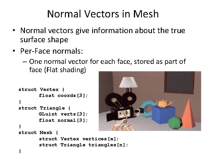
Normal Vectors in Mesh • Normal vectors give information about the true surface shape • Per-Face normals: – One normal vector for each face, stored as part of face (Flat shading) struct Vertex { float coords[3]; } struct Triangle { GLuint verts[3]; float normal[3]; } struct Mesh { struct Vertex vertices[m]; struct Triangle triangles[n]; }

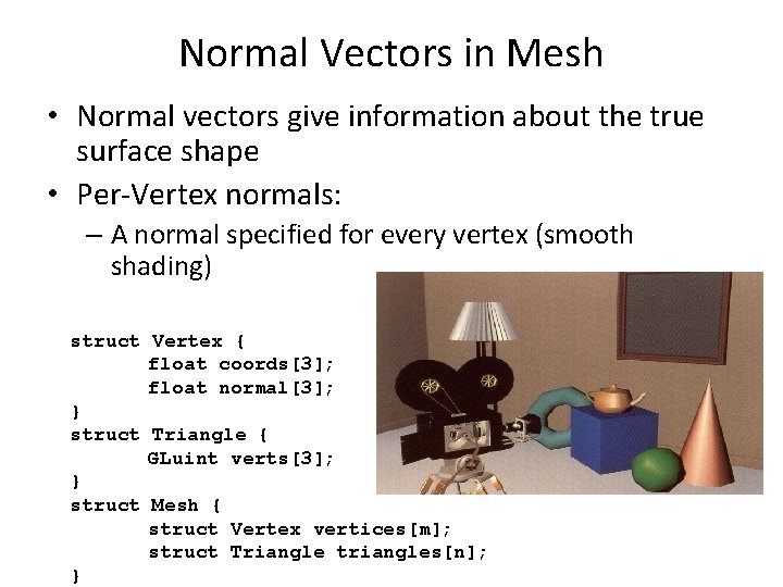
Normal Vectors in Mesh • Normal vectors give information about the true surface shape • Per-Vertex normals: – A normal specified for every vertex (smooth shading) struct Vertex { float coords[3]; float normal[3]; } struct Triangle { GLuint verts[3]; } struct Mesh { struct Vertex vertices[m]; struct Triangle triangles[n]; }

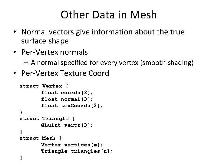
Other Data in Mesh • Normal vectors give information about the true surface shape • Per-Vertex normals: – A normal specified for every vertex (smooth shading) • Per-Vertex Texture Coord struct Vertex { float coords[3]; float normal[3]; float tex. Coords[2]; } struct Triangle { GLuint verts[3]; } struct Mesh { Vertex vertices[m]; Triangle triangles[n]; }

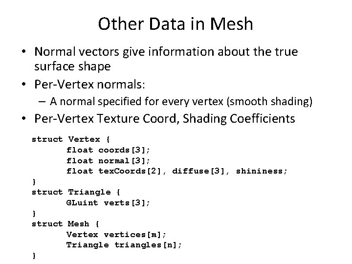
Other Data in Mesh • Normal vectors give information about the true surface shape • Per-Vertex normals: – A normal specified for every vertex (smooth shading) • Per-Vertex Texture Coord, Shading Coefficients struct Vertex { float coords[3]; float normal[3]; float tex. Coords[2], diffuse[3], shininess; } struct Triangle { GLuint verts[3]; } struct Mesh { Vertex vertices[m]; Triangle triangles[n]; }

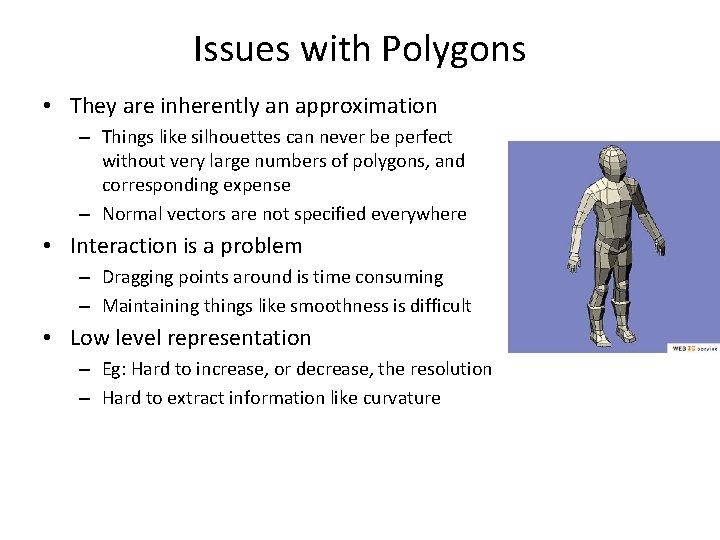
Issues with Polygons • They are inherently an approximation – Things like silhouettes can never be perfect without very large numbers of polygons, and corresponding expense – Normal vectors are not specified everywhere • Interaction is a problem – Dragging points around is time consuming – Maintaining things like smoothness is difficult • Low level representation – Eg: Hard to increase, or decrease, the resolution – Hard to extract information like curvature

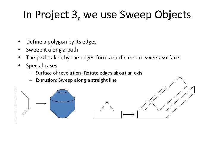
In Project 3, we use Sweep Objects • • Define a polygon by its edges Sweep it along a path The path taken by the edges form a surface - the sweep surface Special cases – Surface of revolution: Rotate edges about an axis – Extrusion: Sweep along a straight line

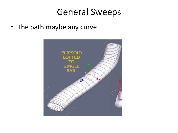
General Sweeps • The path maybe any curve

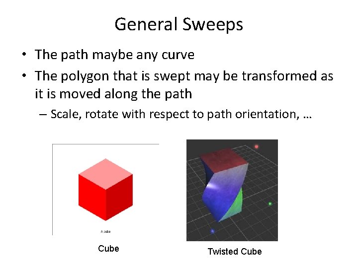
General Sweeps • The path maybe any curve • The polygon that is swept may be transformed as it is moved along the path – Scale, rotate with respect to path orientation, … Cube Twisted Cube

General Sweeps • The path maybe any curve • The polygon that is swept may be transformed as it is moved along the path – Scale, rotate with respect to path orientation, … • One common way to specify is: – Give a poly-line (sequence of line segments) as the path – Give a poly-line as the shape to sweep – Give a transformation to apply at the vertex of each path segment • Texture Coord? • Difficult to avoid self-intersection

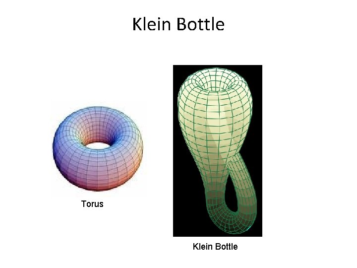
Klein Bottle Torus Klein Bottle

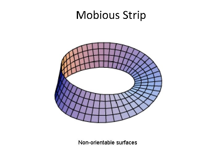
Mobious Strip Non-orientable surfaces

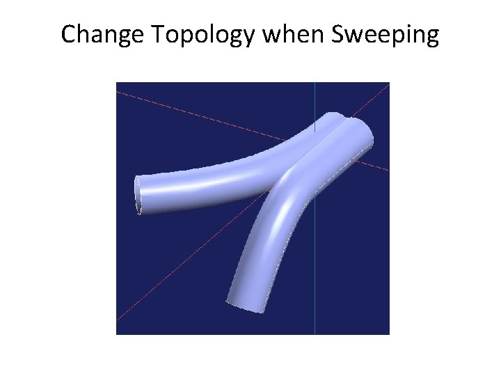
Change Topology when Sweeping

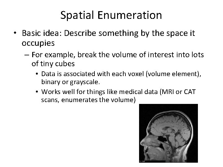
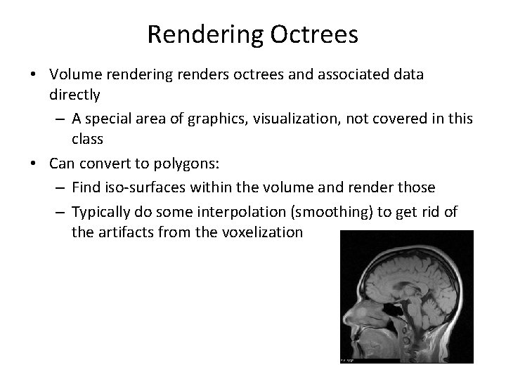
Spatial Enumeration • Basic idea: Describe something by the space it occupies – For example, break the volume of interest into lots of tiny cubes • Data is associated with each voxel (volume element), binary or grayscale. • Works well for things like medical data (MRI or CAT scans, enumerates the volume)

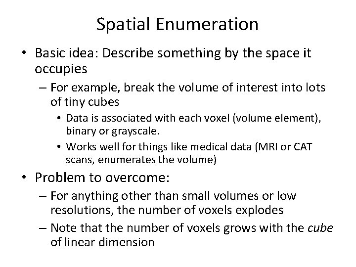
Spatial Enumeration • Basic idea: Describe something by the space it occupies – For example, break the volume of interest into lots of tiny cubes • Data is associated with each voxel (volume element), binary or grayscale. • Works well for things like medical data (MRI or CAT scans, enumerates the volume) • Problem to overcome: – For anything other than small volumes or low resolutions, the number of voxels explodes – Note that the number of voxels grows with the cube of linear dimension

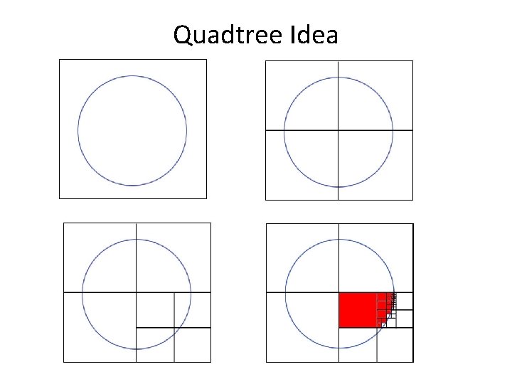
Quadtree Idea

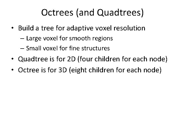
Octrees (and Quadtrees) • Build a tree for adaptive voxel resolution – Large voxel for smooth regions – Small voxel for fine structures • Quadtree is for 2 D (four children for each node) • Octree is for 3 D (eight children for each node)

Rendering Octrees • Volume rendering renders octrees and associated data directly – A special area of graphics, visualization, not covered in this class • Can convert to polygons: – Find iso-surfaces within the volume and render those – Typically do some interpolation (smoothing) to get rid of the artifacts from the voxelization

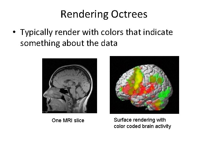
Rendering Octrees • Typically render with colors that indicate something about the data One MRI slice Surface rendering with color coded brain activity

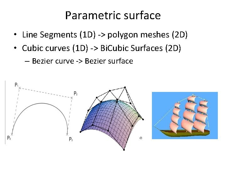
Parametric surface • Line Segments (1 D) -> polygon meshes (2 D) • Cubic curves (1 D) -> Bi. Cubic Surfaces (2 D) – Bezier curve -> Bezier surface

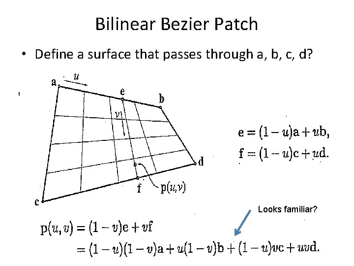
Bilinear Bezier Patch • Define a surface that passes through a, b, c, d? Looks familiar?

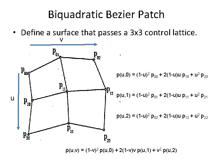
Biquadratic Bezier Patch • Define a surface that passes a 3 x 3 control lattice. v p(u, 0) = (1 -u)2 p 00 + 2(1 -u)u p 10 + u 2 p 20 u p(u, 1) = (1 -u)2 p 01 + 2(1 -u)u p 11 + u 2 p 21 p(u, 2) = (1 -u)2 p 02 + 2(1 -u)u p 12 + u 2 p 22 p(u, v) = (1 -v)2 p(u, 0) + 2(1 -v)v p(u, 1) + v 2 p(u, 2)

Bicubic Bezier Patch • 4 x 4 control points? • Demo: http: //www. nbb. cornell. edu/neurobio/land/Old. S tudent. Projects/cs 49096 to 97/anson/Bezier. Patch. Applet/index. html • Connecting Bezier Patches, demo on the same page.

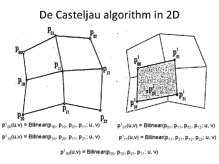
De Casteljau algorithm in 2 D p 100(u, v) = Bilinear(p 00, p 10, p 01, p 11; u, v) p 101(u, v) = Bilinear(p 01, p 11, p 02, p 12; u, v) p 110(u, v) = Bilinear(p 10, p 20, p 11, p 21; u, v) p 111(u, v) = Bilinear(p 11, p 21, p 12, p 22; u, v) p 100(u, v) = Bilinear(p 00, p 10, p 01, p 11; u, v)

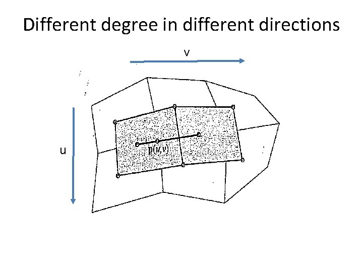
Different degree in different directions v u

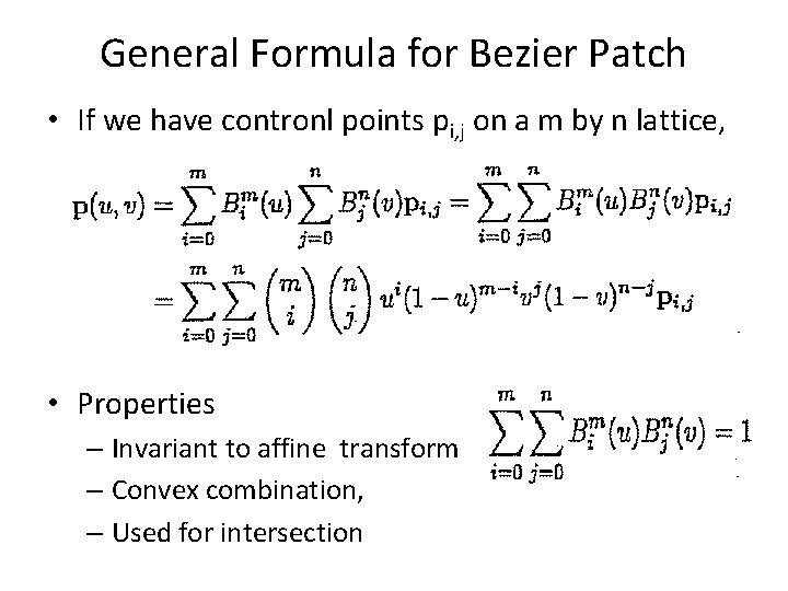
General Formula for Bezier Patch • If we have contronl points pi, j on a m by n lattice, • Properties – Invariant to affine transform – Convex combination, – Used for intersection

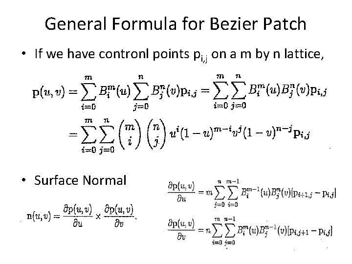
General Formula for Bezier Patch • If we have contronl points pi, j on a m by n lattice, • Surface Normal

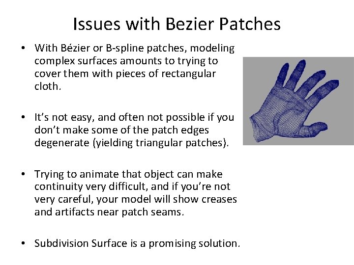
Issues with Bezier Patches • With Bézier or B-spline patches, modeling complex surfaces amounts to trying to cover them with pieces of rectangular cloth. • It’s not easy, and often not possible if you don’t make some of the patch edges degenerate (yielding triangular patches). • Trying to animate that object can make continuity very difficult, and if you’re not very careful, your model will show creases and artifacts near patch seams. • Subdivision Surface is a promising solution.

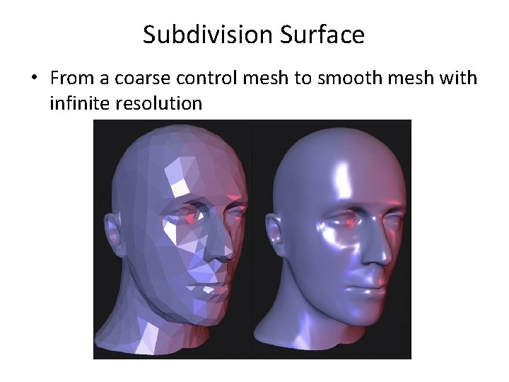
Subdivision Surface • From a coarse control mesh to smooth mesh with infinite resolution

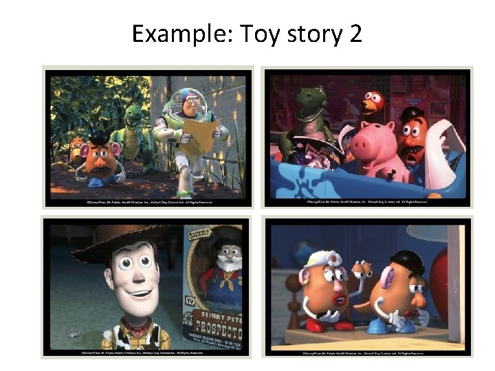
Example: Toy story 2

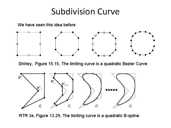
Subdivision Curve We have seen this idea before Shirley, Figure 15. 15, The limiting curve is a quadratic Bezier Curve RTR 3 e, Figure 13. 29, The limiting curve is a quadratic B-spline

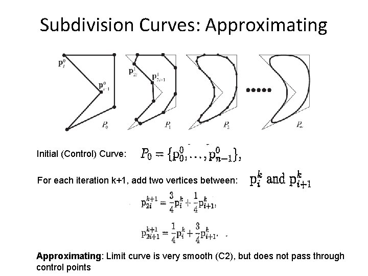
Subdivision Curves: Approximating Initial (Control) Curve: For each iteration k+1, add two vertices between: Approximating: Limit curve is very smooth (C 2), but does not pass through control points

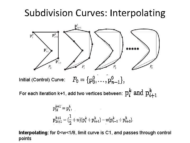
Subdivision Curves: Interpolating Initial (Control) Curve: For each iteration k+1, add two vertices between: Interpolating: for 0<w<1/8, limit curve is C 1, and passes through control points

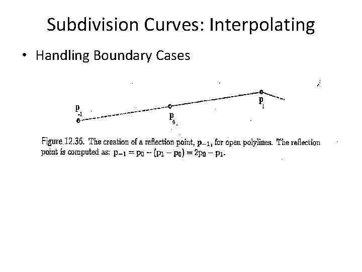
Subdivision Curves: Interpolating • Handling Boundary Cases

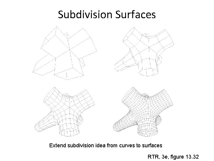
Subdivision Surfaces Extend subdivision idea from curves to surfaces RTR, 3 e, figure 13. 32

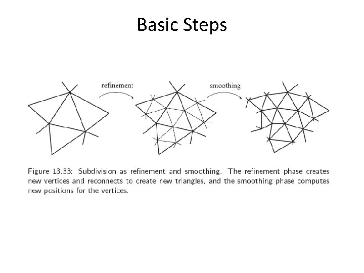
Basic Steps

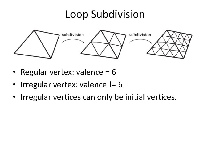
Loop Subdivision • Regular vertex: valence = 6 • Irregular vertex: valence != 6 • Irregular vertices can only be initial vertices.

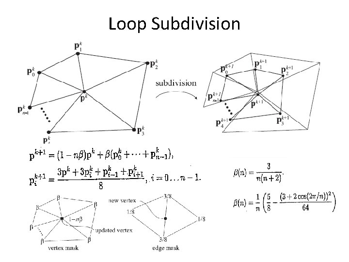
Loop Subdivision

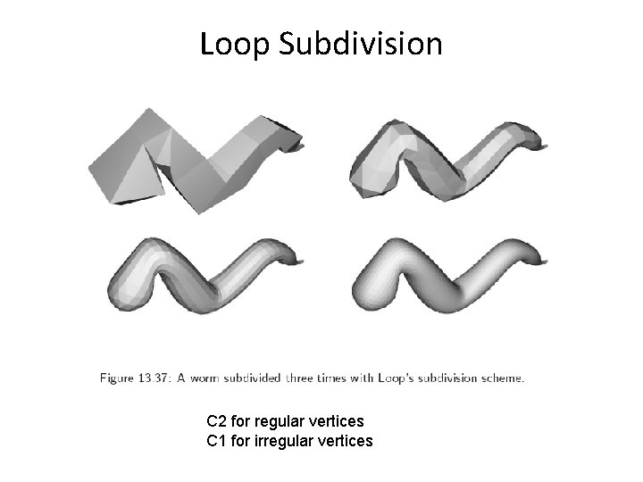
Loop Subdivision C 2 for regular vertices C 1 for irregular vertices

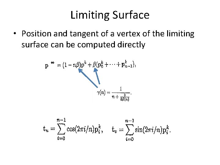
Limiting Surface • Position and tangent of a vertex of the limiting surface can be computed directly ∞

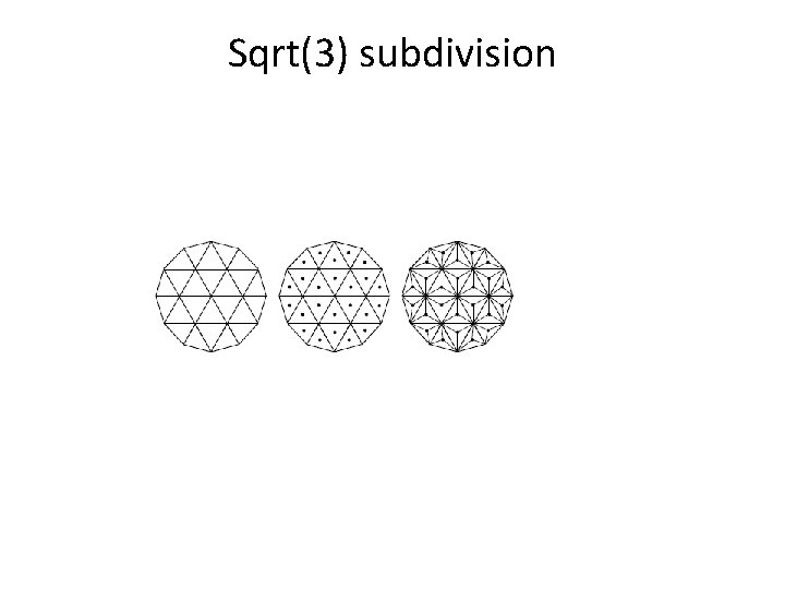
Sqrt(3) subdivision

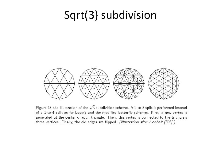
Sqrt(3) subdivision

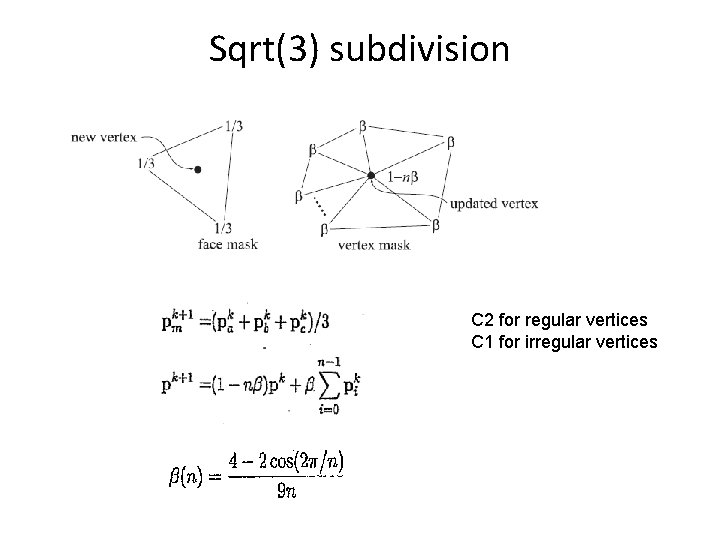
Sqrt(3) subdivision C 2 for regular vertices C 1 for irregular vertices

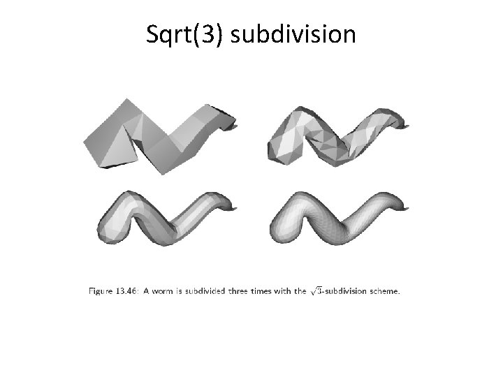
Sqrt(3) subdivision

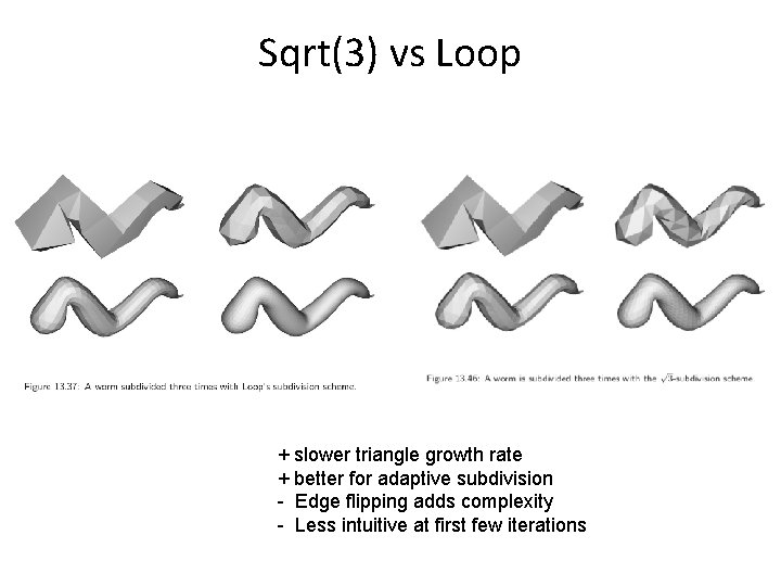
Sqrt(3) vs Loop + slower triangle growth rate + better for adaptive subdivision - Edge flipping adds complexity - Less intuitive at first few iterations