CS 559 Computer Graphics Lecture 15 Hierarchical Modeling

CS 559: Computer Graphics Lecture 15: Hierarchical Modeling and Shading Li Zhang Spring 2008

Today • Finish transformation in Open. GL • Lighting • Reading – Shirley, Ch 9. 1, 9. 2

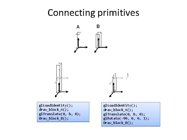
Connecting primitives A gl. Load. Identity(); draw_block_A(); gl. Translate(0, h, 0); Draw_block_B(); B gl. Load. Identity(); draw_block_A(); gl. Translate(0, h, 0); gl. Rotate(-90, 0, 0, 1); Draw_block_B();

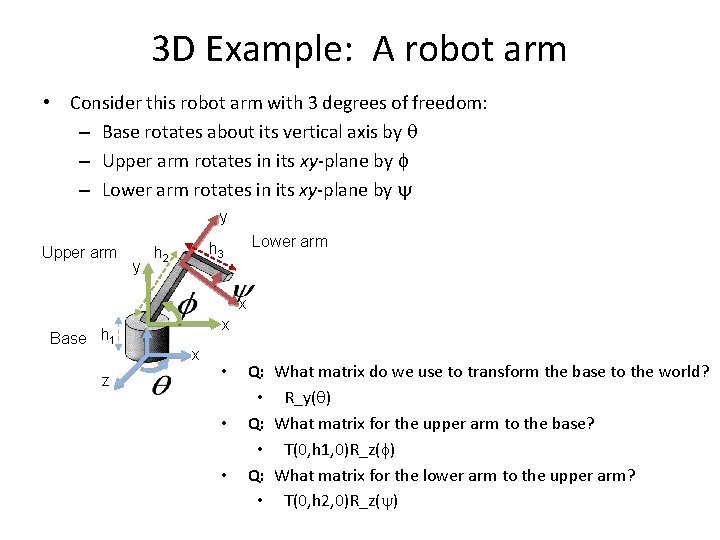
3 D Example: A robot arm • Consider this robot arm with 3 degrees of freedom: – Base rotates about its vertical axis by – Upper arm rotates in its xy-plane by – Lower arm rotates in its xy-plane by y Upper arm y Lower arm h 3 h 2 x Base h 1 z x x • • • Q: What matrix do we use to transform the base to the world? • R_y( ) Q: What matrix for the upper arm to the base? • T(0, h 1, 0)R_z( ) Q: What matrix for the lower arm to the upper arm? • T(0, h 2, 0)R_z( )

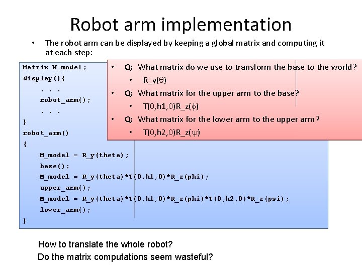
Robot arm implementation • The robot arm can be displayed by keeping a global matrix and computing it at each step: Matrix M_model; • display(){. . . robot_arm(); . . . } robot_arm() • • Q: What matrix do we use to transform the base to the world? • R_y( ) Q: What matrix for the upper arm to the base? • T(0, h 1, 0)R_z( ) Q: What matrix for the lower arm to the upper arm? • T(0, h 2, 0)R_z( ) { M_model = R_y(theta); base(); M_model = R_y(theta)*T(0, h 1, 0)*R_z(phi); upper_arm(); M_model = R_y(theta)*T(0, h 1, 0)*R_z(phi)*T(0, h 2, 0)*R_z(psi); lower_arm(); } How to translate the whole robot? Do the matrix computations seem wasteful?

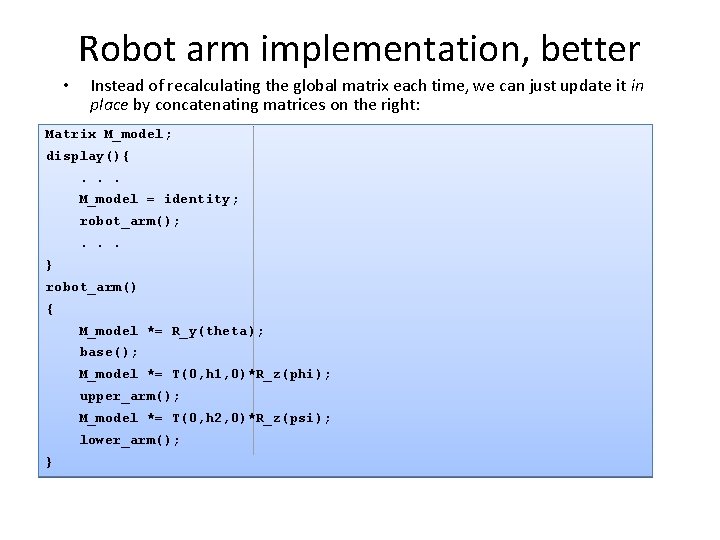
Robot arm implementation, better • Instead of recalculating the global matrix each time, we can just update it in place by concatenating matrices on the right: Matrix M_model; display(){. . . M_model = identity; robot_arm(); . . . } robot_arm() { M_model *= R_y(theta); base(); M_model *= T(0, h 1, 0)*R_z(phi); upper_arm(); M_model *= T(0, h 2, 0)*R_z(psi); lower_arm(); }

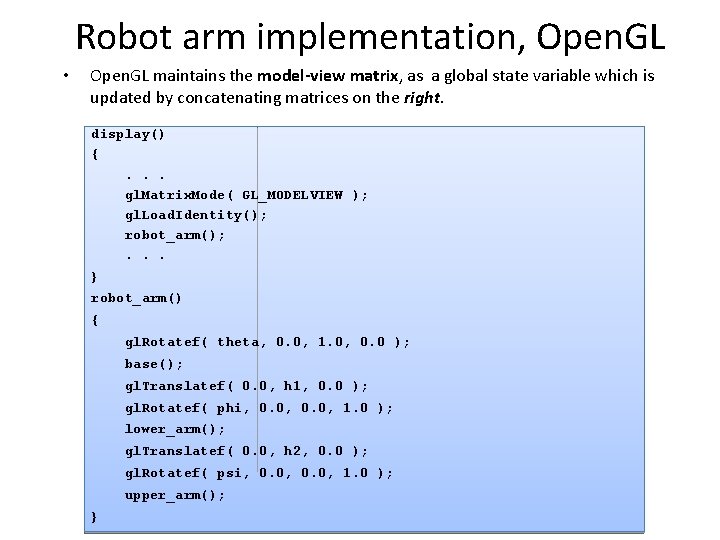
Robot arm implementation, Open. GL • Open. GL maintains the model-view matrix, as a global state variable which is updated by concatenating matrices on the right. display() {. . . gl. Matrix. Mode( GL_MODELVIEW ); gl. Load. Identity(); robot_arm(); . . . } robot_arm() { gl. Rotatef( theta, 0. 0, 1. 0, 0. 0 ); base(); gl. Translatef( 0. 0, h 1, 0. 0 ); gl. Rotatef( phi, 0. 0, 1. 0 ); lower_arm(); gl. Translatef( 0. 0, h 2, 0. 0 ); gl. Rotatef( psi, 0. 0, 1. 0 ); upper_arm(); }

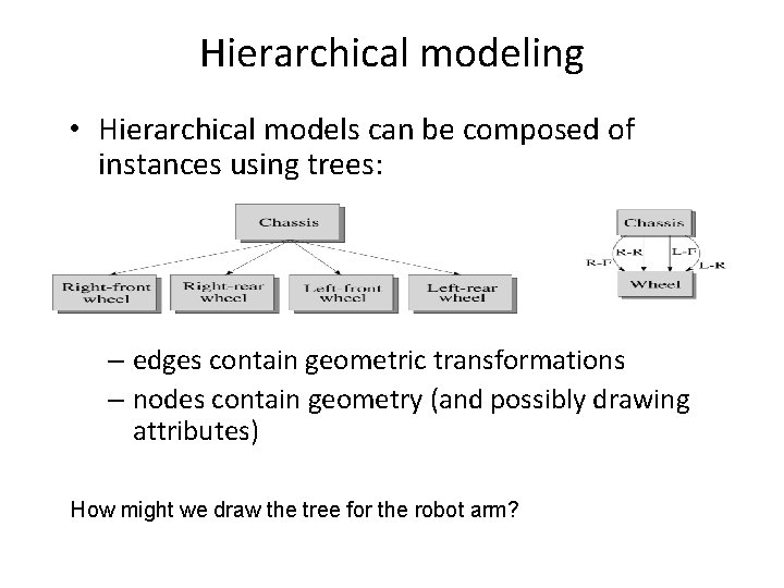
Hierarchical modeling • Hierarchical models can be composed of instances using trees: – edges contain geometric transformations – nodes contain geometry (and possibly drawing attributes) How might we draw the tree for the robot arm?

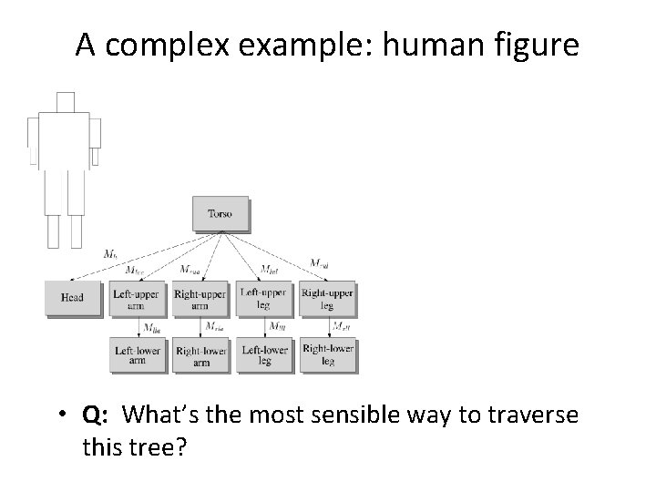
A complex example: human figure • Q: What’s the most sensible way to traverse this tree?

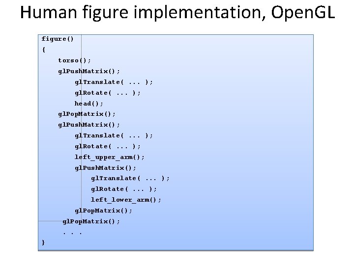
Human figure implementation, Open. GL figure() { torso(); gl. Push. Matrix(); gl. Translate(. . . ); gl. Rotate(. . . ); head(); gl. Pop. Matrix(); gl. Push. Matrix(); gl. Translate(. . . ); gl. Rotate(. . . ); left_upper_arm(); gl. Push. Matrix(); gl. Translate(. . . ); gl. Rotate(. . . ); left_lower_arm(); gl. Pop. Matrix(); . . . }

So far… • We’ve talked exclusively about geometry. – What is the shape of an object? • gl. Begin() … gl. End() – How do I place it in a virtual 3 D space? • gl. Matrix. Mode() … – How to change viewpoints • glu. Look. At() – How do I know which pixels it covers? • Rasterization – How do I know which of the pixels I should actually draw? • Z-buffer, BSP

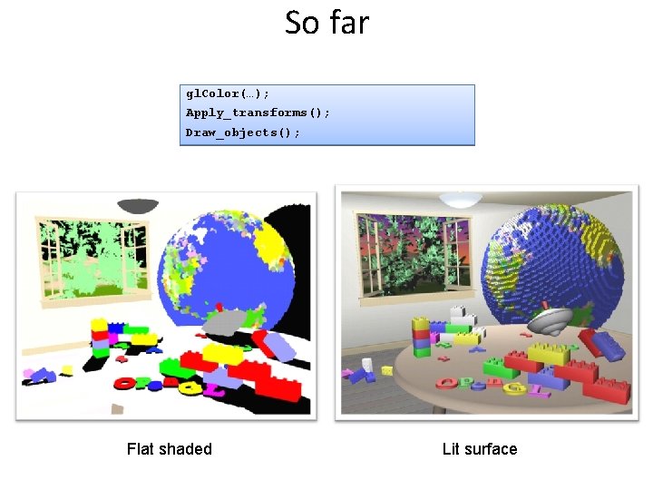
So far gl. Color(…); Apply_transforms(); Draw_objects(); Flat shaded Lit surface

Next… • Once we know geometry, we have to ask one more important question: – To what value do I set each pixel? • Answering this question is the job of the shading model. • Other names: – Lighting model – Light reflection model – Local illumination model – Reflectance model – BRDF

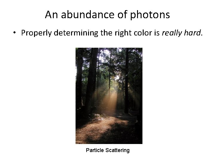
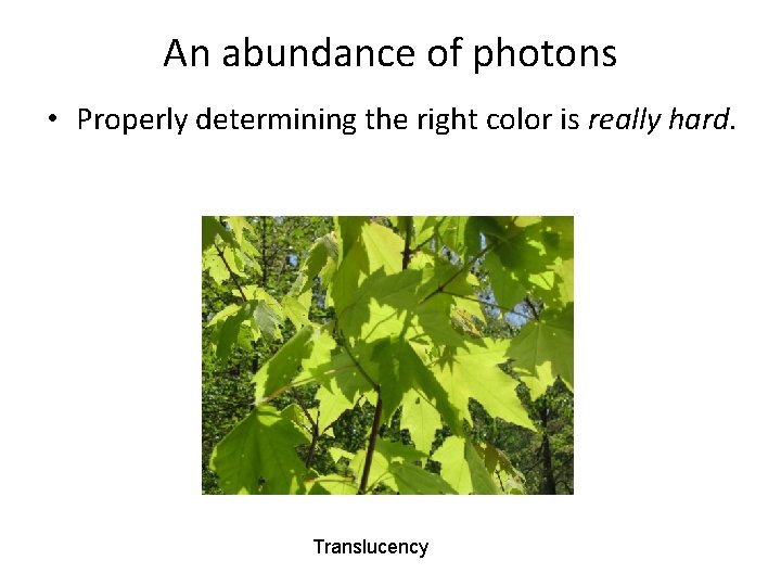
An abundance of photons • Properly determining the right color is really hard. Particle Scattering

An abundance of photons • Properly determining the right color is really hard. Translucency

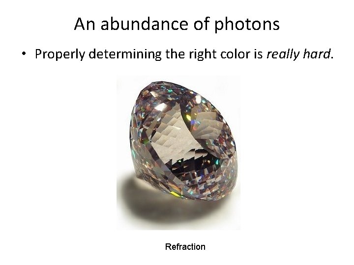
An abundance of photons • Properly determining the right color is really hard. Refraction

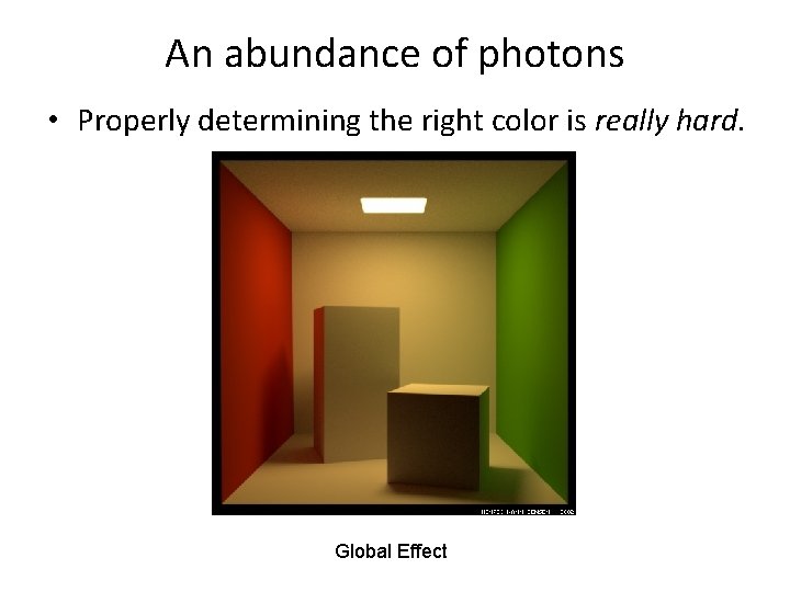
An abundance of photons • Properly determining the right color is really hard. Global Effect

Our problem • We’re going to build up to an approximation of reality called the Phong illumination model. • It has the following characteristics: – not physically based – gives a “first-order” approximation to physical light reflection – very fast – widely used • In addition, we will assume local illumination, i. e. , light goes: light source -> surface -> viewer. • No interreflections, no shadows.

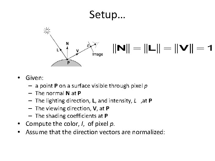
Setup… • Given: – – – a point P on a surface visible through pixel p The normal N at P The lighting direction, L, and intensity, L , at P The viewing direction, V, at P The shading coefficients at P • Compute the color, I, of pixel p. • Assume that the direction vectors are normalized:

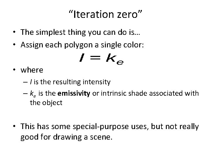
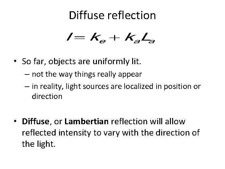
“Iteration zero” • The simplest thing you can do is… • Assign each polygon a single color: • where – I is the resulting intensity – ke is the emissivity or intrinsic shade associated with the object • This has some special-purpose uses, but not really good for drawing a scene.

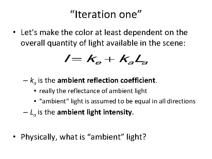
“Iteration one” • Let’s make the color at least dependent on the overall quantity of light available in the scene: – ka is the ambient reflection coefficient. • really the reflectance of ambient light • “ambient” light is assumed to be equal in all directions – La is the ambient light intensity. • Physically, what is “ambient” light?

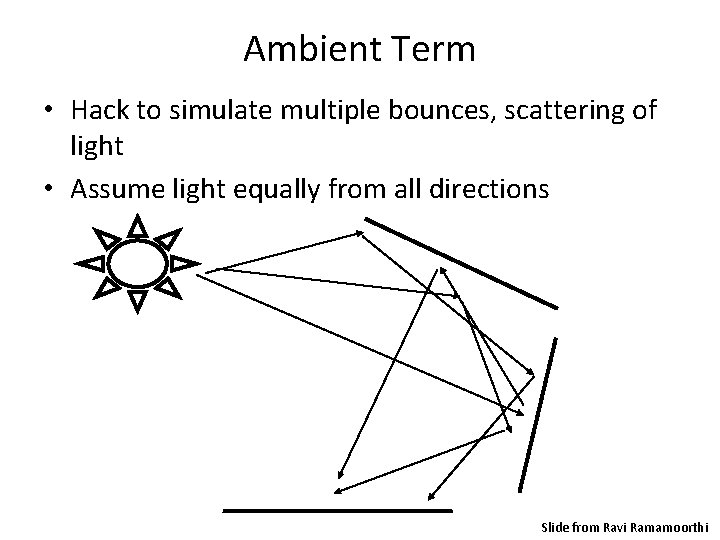
Ambient Term • Hack to simulate multiple bounces, scattering of light • Assume light equally from all directions Slide from Ravi Ramamoorthi

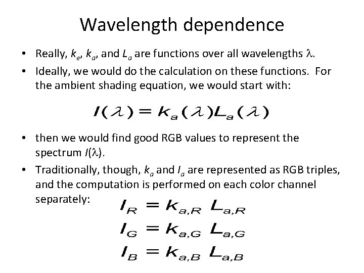
Wavelength dependence • Really, ke, ka, and La are functions over all wavelengths . • Ideally, we would do the calculation on these functions. For the ambient shading equation, we would start with: • then we would find good RGB values to represent the spectrum I( ). • Traditionally, though, ka and Ia are represented as RGB triples, and the computation is performed on each color channel separately:

Diffuse reflection • So far, objects are uniformly lit. – not the way things really appear – in reality, light sources are localized in position or direction • Diffuse, or Lambertian reflection will allow reflected intensity to vary with the direction of the light.

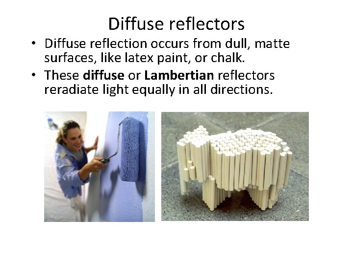
Diffuse reflectors • Diffuse reflection occurs from dull, matte surfaces, like latex paint, or chalk. • These diffuse or Lambertian reflectors reradiate light equally in all directions.

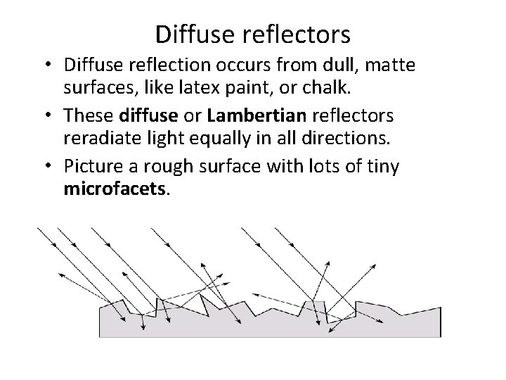
Diffuse reflectors • Diffuse reflection occurs from dull, matte surfaces, like latex paint, or chalk. • These diffuse or Lambertian reflectors reradiate light equally in all directions. • Picture a rough surface with lots of tiny microfacets.

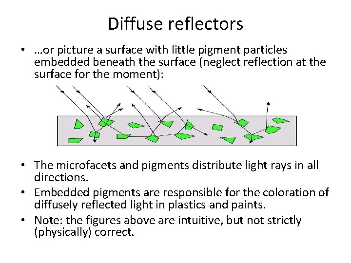
Diffuse reflectors • …or picture a surface with little pigment particles embedded beneath the surface (neglect reflection at the surface for the moment): • The microfacets and pigments distribute light rays in all directions. • Embedded pigments are responsible for the coloration of diffusely reflected light in plastics and paints. • Note: the figures above are intuitive, but not strictly (physically) correct.

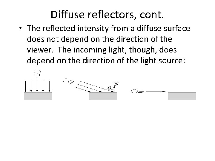
Diffuse reflectors, cont. • The reflected intensity from a diffuse surface does not depend on the direction of the viewer. The incoming light, though, does depend on the direction of the light source:

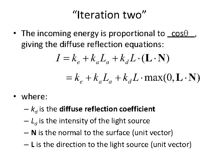
“Iteration two” • The incoming energy is proportional to cos , giving the diffuse reflection equations: • where: – kd is the diffuse reflection coefficient – Ld is the intensity of the light source – N is the normal to the surface (unit vector) – L is the direction to the light source (unit vector)