CS 558 COMPUTER VISION Lecture VIII Single View

CS 558 COMPUTER VISION Lecture VIII: Single View and Epipolar Geometry Slide adapted from S. Lazebnik

OUTLINE Single view geometry Epiploar geometry

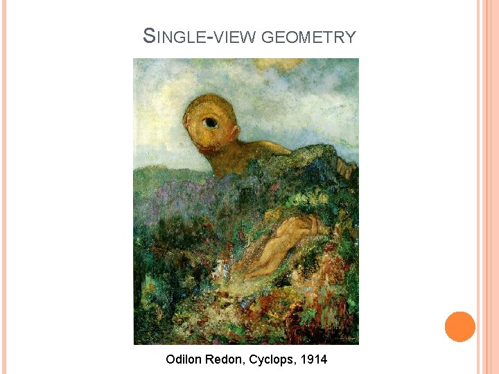
SINGLE-VIEW GEOMETRY Odilon Redon, Cyclops, 1914

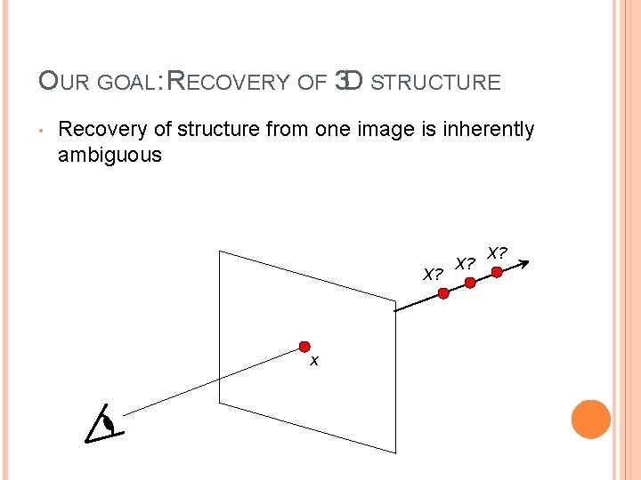
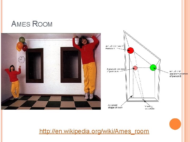
OUR GOAL: RECOVERY OF 3 D STRUCTURE • Recovery of structure from one image is inherently ambiguous X? x X?

OUR GOAL: RECOVERY OF 3 D STRUCTURE • Recovery of structure from one image is inherently ambiguous

OUR GOAL: RECOVERY OF 3 D STRUCTURE • Recovery of structure from one image is inherently ambiguous

AMES ROOM http: //en. wikipedia. org/wiki/Ames_room

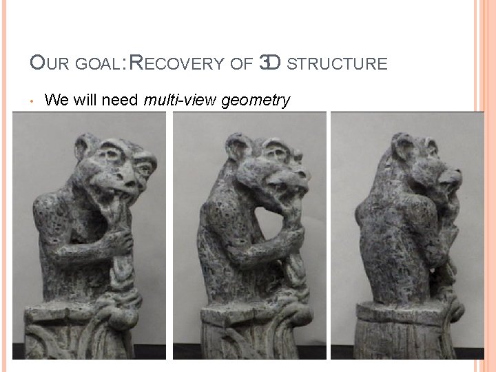
OUR GOAL: RECOVERY OF 3 D STRUCTURE • We will need multi-view geometry

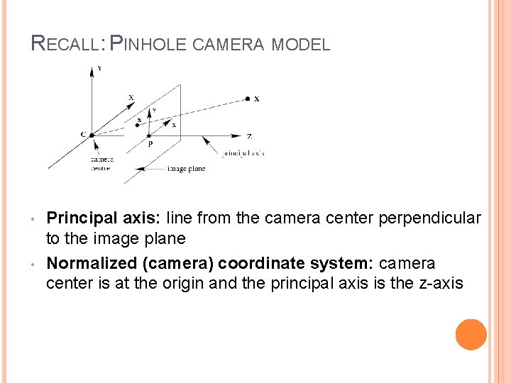
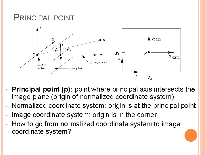
RECALL: PINHOLE CAMERA MODEL • • Principal axis: line from the camera center perpendicular to the image plane Normalized (camera) coordinate system: camera center is at the origin and the principal axis is the z-axis

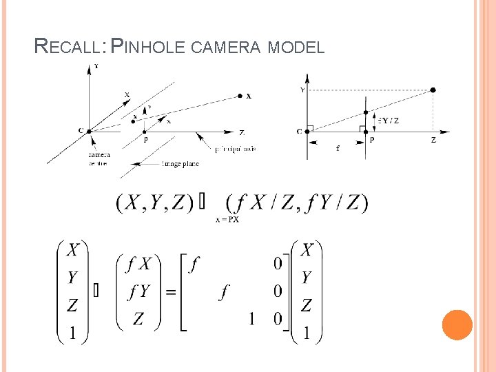
RECALL: PINHOLE CAMERA MODEL

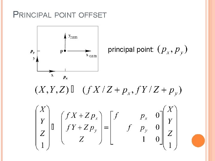
PRINCIPAL POINT py px • • Principal point (p): point where principal axis intersects the image plane (origin of normalized coordinate system) Normalized coordinate system: origin is at the principal point Image coordinate system: origin is in the corner How to go from normalized coordinate system to image coordinate system?

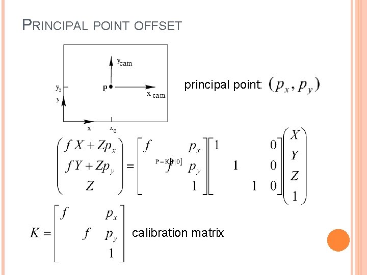
PRINCIPAL POINT OFFSET principal point: py px

PRINCIPAL POINT OFFSET principal point: calibration matrix

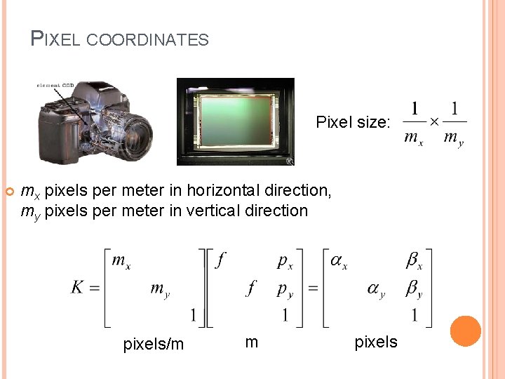
PIXEL COORDINATES Pixel size: mx pixels per meter in horizontal direction, my pixels per meter in vertical direction pixels/m m pixels

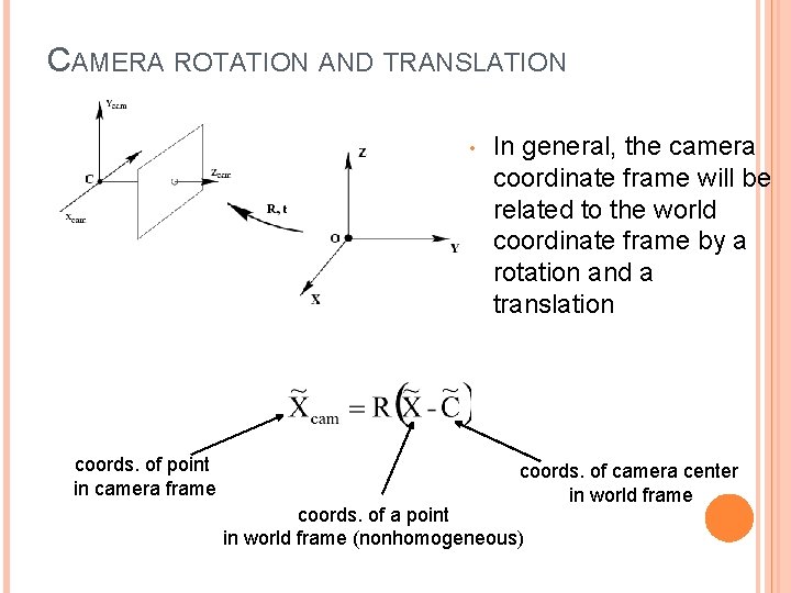
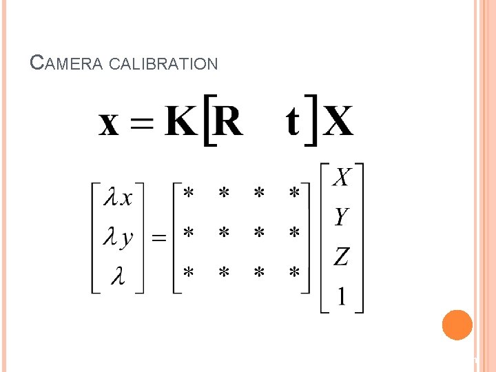
CAMERA ROTATION AND TRANSLATION • coords. of point in camera frame In general, the camera coordinate frame will be related to the world coordinate frame by a rotation and a translation coords. of camera center in world frame coords. of a point in world frame (nonhomogeneous)

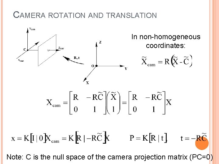
CAMERA ROTATION AND TRANSLATION In non-homogeneous coordinates: Note: C is the null space of the camera projection matrix (PC=0)

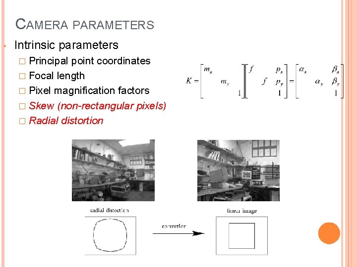
CAMERA PARAMETERS • Intrinsic parameters � Principal point coordinates � Focal length � Pixel magnification factors � Skew (non-rectangular pixels) � Radial distortion

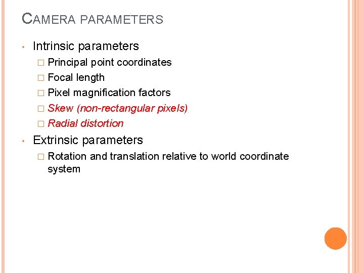
CAMERA PARAMETERS • Intrinsic parameters � Principal point coordinates � Focal length � Pixel magnification factors � Skew (non-rectangular pixels) � Radial distortion • Extrinsic parameters � Rotation system and translation relative to world coordinate

CAMERA CALIBRATION Source: D. Hoiem

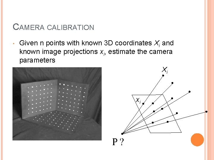
CAMERA CALIBRATION • Given n points with known 3 D coordinates Xi and known image projections xi, estimate the camera parameters Xi xi

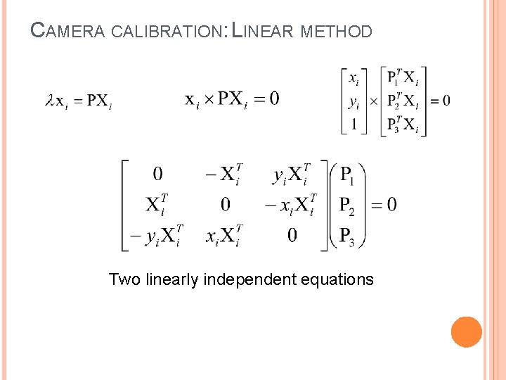
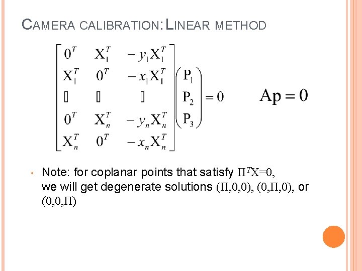
CAMERA CALIBRATION: LINEAR METHOD Two linearly independent equations

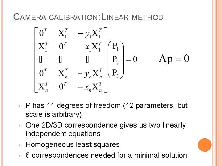
CAMERA CALIBRATION: LINEAR METHOD • • P has 11 degrees of freedom (12 parameters, but scale is arbitrary) One 2 D/3 D correspondence gives us two linearly independent equations Homogeneous least squares 6 correspondences needed for a minimal solution

CAMERA CALIBRATION: LINEAR METHOD • Note: for coplanar points that satisfy ΠTX=0, we will get degenerate solutions (Π, 0, 0), (0, Π, 0), or (0, 0, Π)

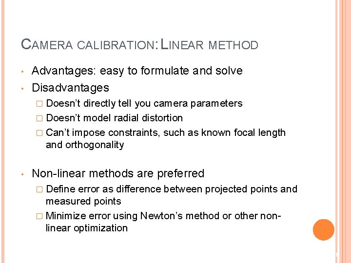
CAMERA CALIBRATION: LINEAR METHOD • • Advantages: easy to formulate and solve Disadvantages � Doesn’t directly tell you camera parameters � Doesn’t model radial distortion � Can’t impose constraints, such as known focal length and orthogonality • Non-linear methods are preferred � Define error as difference between projected points and measured points � Minimize error using Newton’s method or other nonlinear optimization Source: D. Hoiem

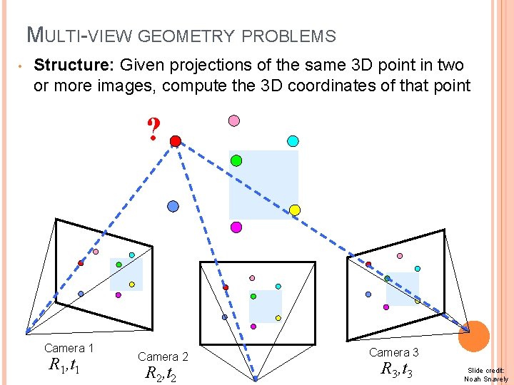
MULTI-VIEW GEOMETRY PROBLEMS • Structure: Given projections of the same 3 D point in two or more images, compute the 3 D coordinates of that point ? Camera 1 R 1, t 1 Camera 2 R 2, t 2 Camera 3 R 3, t 3 Slide credit: Noah Snavely

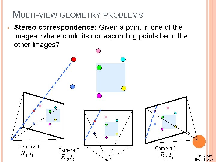
MULTI-VIEW GEOMETRY PROBLEMS • Stereo correspondence: Given a point in one of the images, where could its corresponding points be in the other images? Camera 1 R 1, t 1 Camera 2 R 2, t 2 Camera 3 R 3, t 3 Slide credit: Noah Snavely

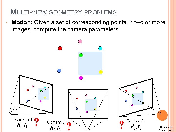
MULTI-VIEW GEOMETRY PROBLEMS • Motion: Given a set of corresponding points in two or more images, compute the camera parameters Camera 1 R 1, t 1 ? Camera 2 R 2, t 2 ? ? Camera 3 R 3, t 3 Slide credit: Noah Snavely

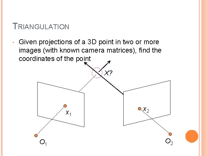
TRIANGULATION • Given projections of a 3 D point in two or more images (with known camera matrices), find the coordinates of the point X? x 1 O 1 x 2 O 2

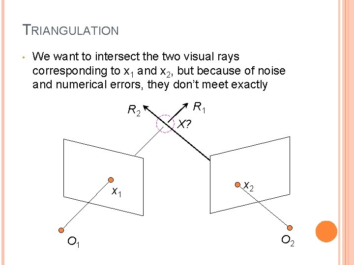
TRIANGULATION • We want to intersect the two visual rays corresponding to x 1 and x 2, but because of noise and numerical errors, they don’t meet exactly R 2 x 1 O 1 R 1 X? x 2 O 2

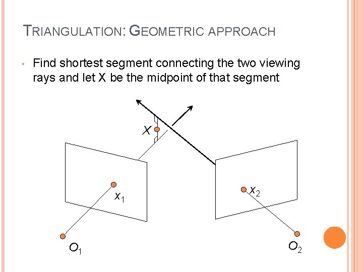
TRIANGULATION: GEOMETRIC APPROACH • Find shortest segment connecting the two viewing rays and let X be the midpoint of that segment X x 1 O 1 x 2 O 2

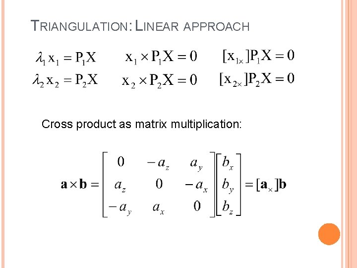
TRIANGULATION: LINEAR APPROACH Cross product as matrix multiplication:

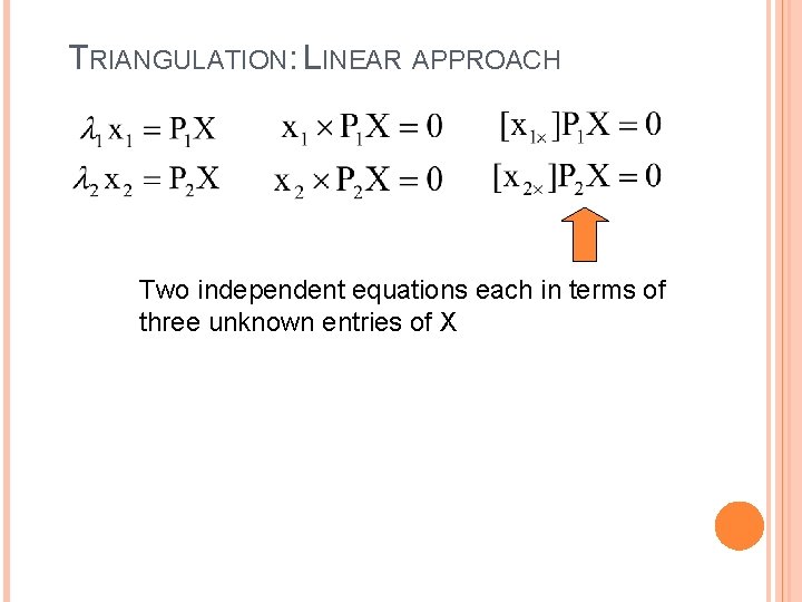
TRIANGULATION: LINEAR APPROACH Two independent equations each in terms of three unknown entries of X

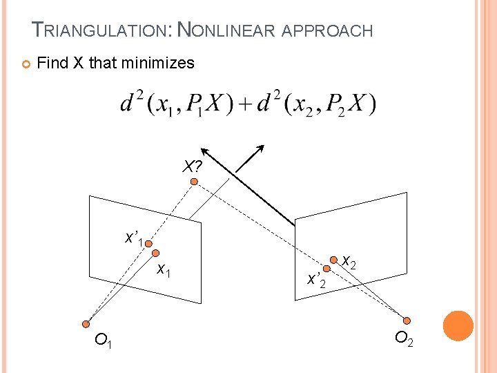
TRIANGULATION: NONLINEAR APPROACH Find X that minimizes X? x’ 1 x 1 O 1 x’ 2 x 2 O 2

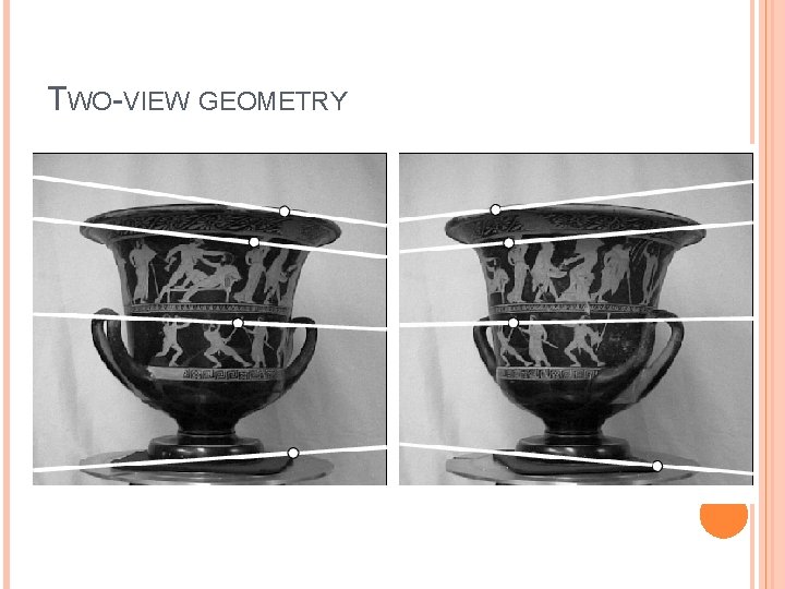
TWO-VIEW GEOMETRY

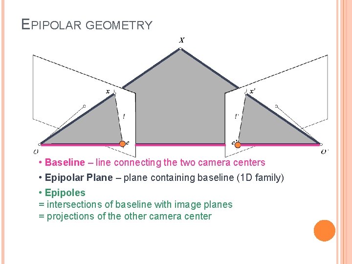
EPIPOLAR GEOMETRY X x x’ • Baseline – line connecting the two camera centers • Epipolar Plane – plane containing baseline (1 D family) • Epipoles = intersections of baseline with image planes = projections of the other camera center

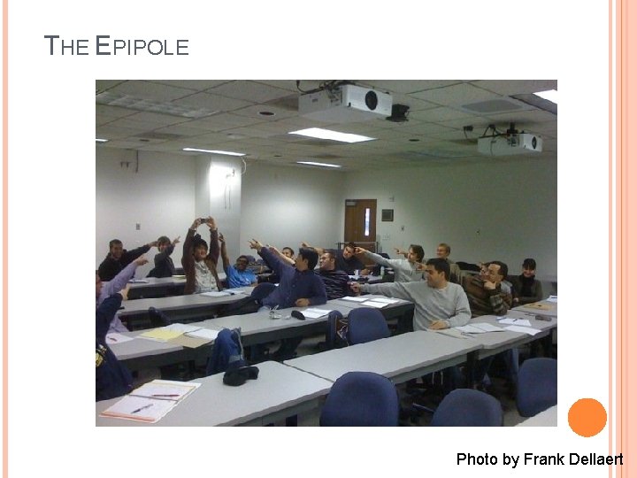
THE EPIPOLE Photo by Frank Dellaert

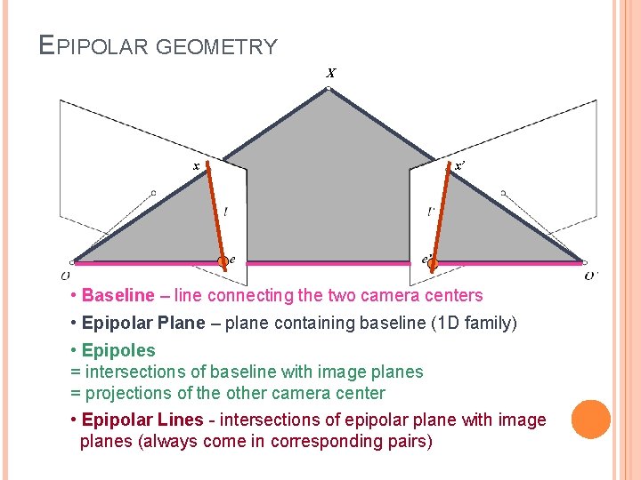
EPIPOLAR GEOMETRY X x x’ • Baseline – line connecting the two camera centers • Epipolar Plane – plane containing baseline (1 D family) • Epipoles = intersections of baseline with image planes = projections of the other camera center • Epipolar Lines - intersections of epipolar plane with image planes (always come in corresponding pairs)

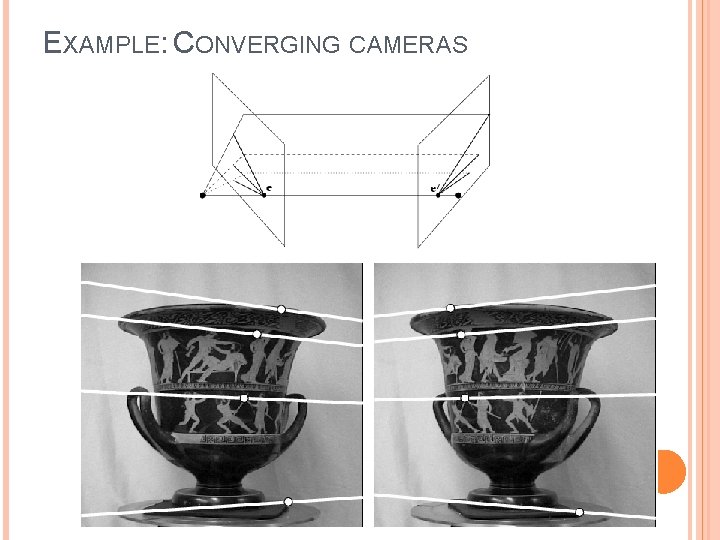
EXAMPLE: CONVERGING CAMERAS

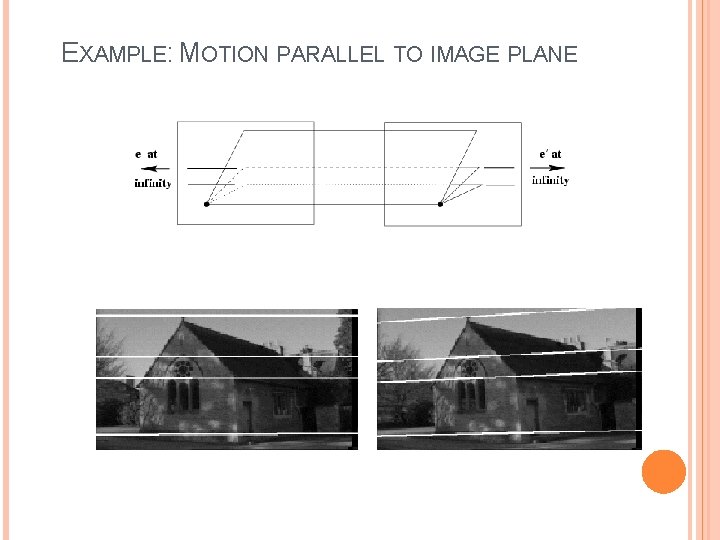
EXAMPLE: MOTION PARALLEL TO IMAGE PLANE

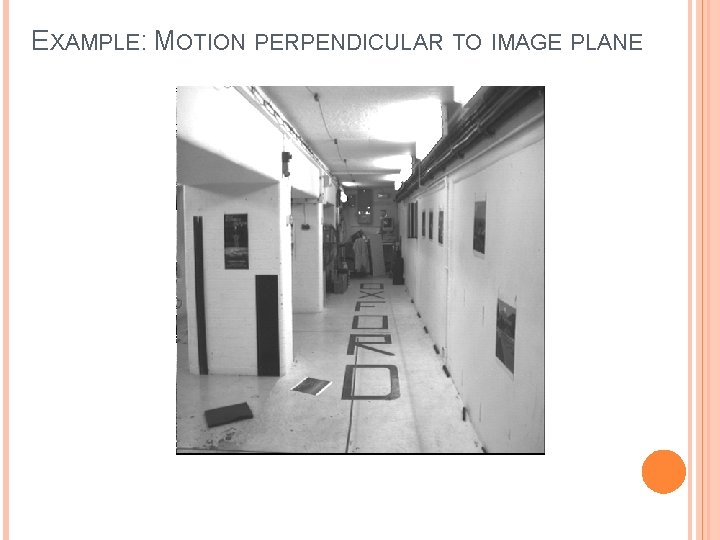
EXAMPLE: MOTION PERPENDICULAR TO IMAGE PLANE

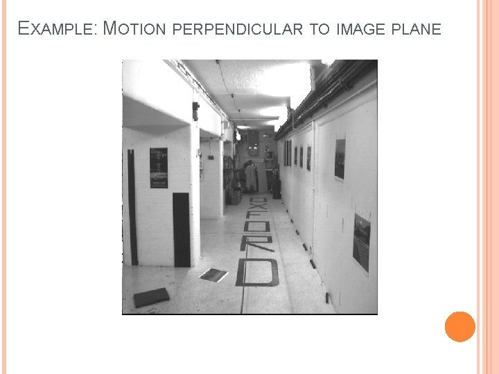
EXAMPLE: MOTION PERPENDICULAR TO IMAGE PLANE

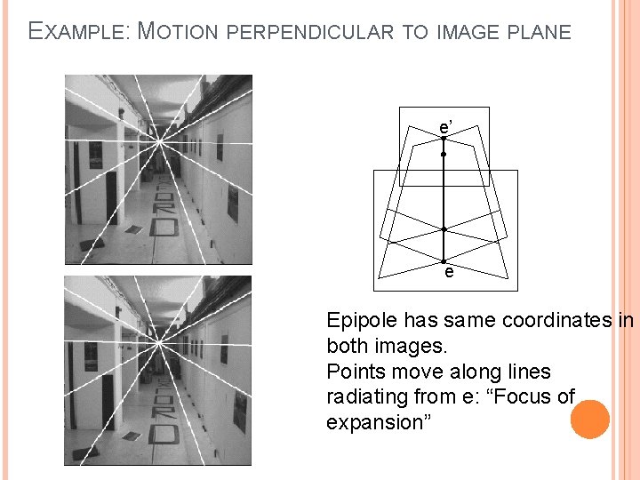
EXAMPLE: MOTION PERPENDICULAR TO IMAGE PLANE e’ e Epipole has same coordinates in both images. Points move along lines radiating from e: “Focus of expansion”

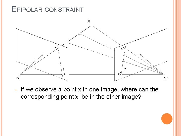
EPIPOLAR CONSTRAINT X x • x’ If we observe a point x in one image, where can the corresponding point x’ be in the other image?

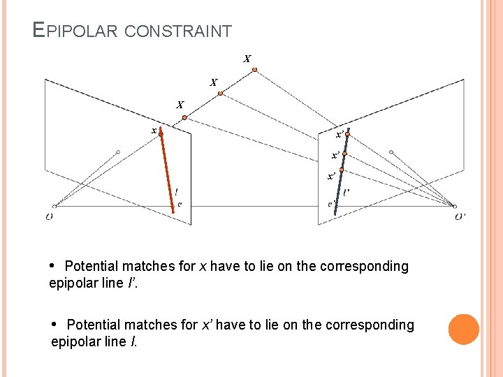
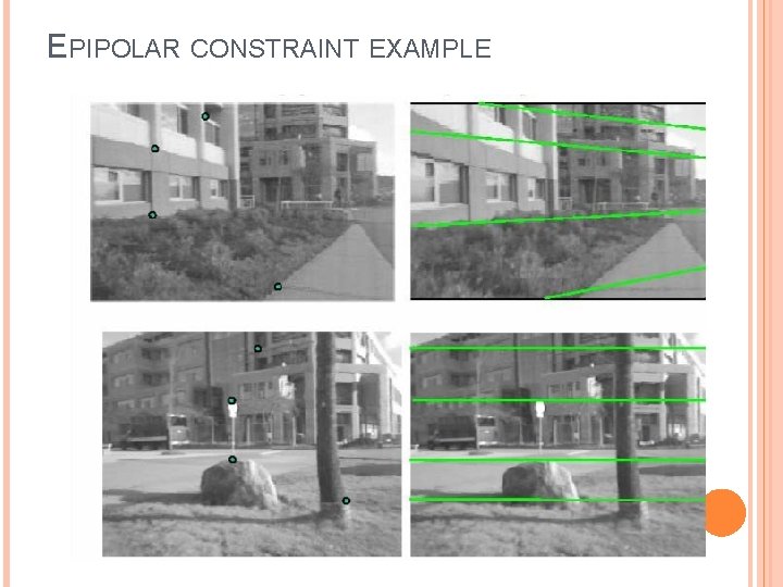
EPIPOLAR CONSTRAINT X X X x x’ x’ x’ • Potential matches for x have to lie on the corresponding epipolar line l’. • Potential matches for x’ have to lie on the corresponding epipolar line l.

EPIPOLAR CONSTRAINT EXAMPLE

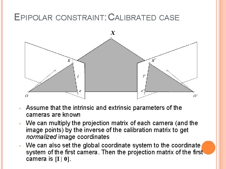
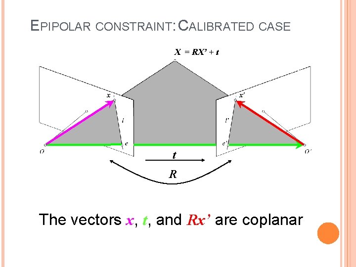
EPIPOLAR CONSTRAINT: CALIBRATED CASE X x • • • x’ Assume that the intrinsic and extrinsic parameters of the cameras are known We can multiply the projection matrix of each camera (and the image points) by the inverse of the calibration matrix to get normalized image coordinates We can also set the global coordinate system to the coordinate system of the first camera. Then the projection matrix of the first camera is [I | 0].

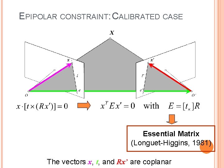
EPIPOLAR CONSTRAINT: CALIBRATED CASE X = RX’ + t x x’ t R The vectors x, t, and Rx’ are coplanar

EPIPOLAR CONSTRAINT: CALIBRATED CASE X x x’ Essential Matrix (Longuet-Higgins, 1981) The vectors x, t, and Rx’ are coplanar

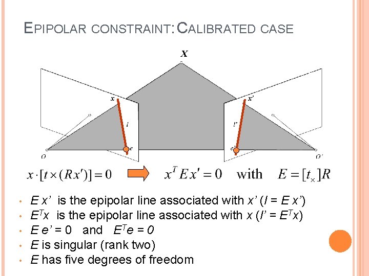
EPIPOLAR CONSTRAINT: CALIBRATED CASE X x • • • x’ E x’ is the epipolar line associated with x’ (l = E x’) ETx is the epipolar line associated with x (l’ = ETx) E e’ = 0 and ETe = 0 E is singular (rank two) E has five degrees of freedom

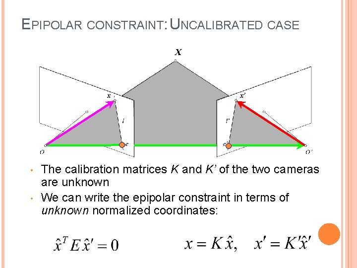
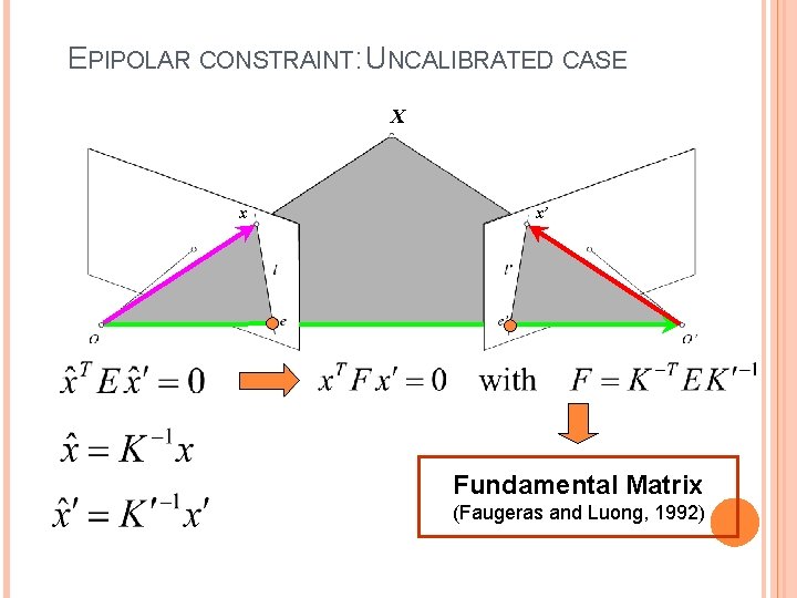
EPIPOLAR CONSTRAINT: UNCALIBRATED CASE X x • • x’ The calibration matrices K and K’ of the two cameras are unknown We can write the epipolar constraint in terms of unknown normalized coordinates:

EPIPOLAR CONSTRAINT: UNCALIBRATED CASE X x x’ Fundamental Matrix (Faugeras and Luong, 1992)

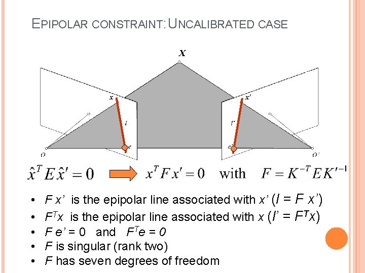
EPIPOLAR CONSTRAINT: UNCALIBRATED CASE X x • • • x’ F x’ is the epipolar line associated with x’ (l = F x’) FTx is the epipolar line associated with x (l’ = FTx) F e’ = 0 and FTe = 0 F is singular (rank two) F has seven degrees of freedom

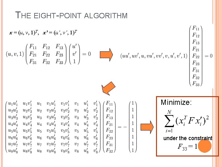
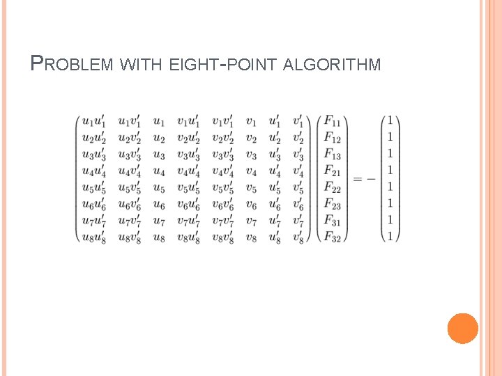
THE EIGHT-POINT ALGORITHM x = (u, v, 1)T, x’ = (u’, v’, 1)T Minimize: under the constraint F 33 = 1

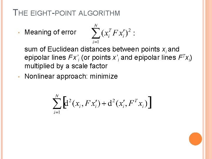
THE EIGHT-POINT ALGORITHM • Meaning of error • sum of Euclidean distances between points xi and epipolar lines F x’i (or points x’i and epipolar lines FTxi) multiplied by a scale factor Nonlinear approach: minimize

PROBLEM WITH EIGHT-POINT ALGORITHM

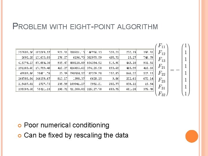
PROBLEM WITH EIGHT-POINT ALGORITHM Poor numerical conditioning Can be fixed by rescaling the data

THE NORMALIZED EIGHT-POINT ALGORITHM (Hartley, 1995) • • Center the image data at the origin, and scale it so the mean squared distance between the origin and the data points is 2 pixels Use the eight-point algorithm to compute F from the normalized points Enforce the rank-2 constraint (for example, take SVD of F and throw out the smallest singular value) Transform fundamental matrix back to original units: if T and T’ are the normalizing transformations in the two images, than the fundamental matrix in original coordinates is TT F T’

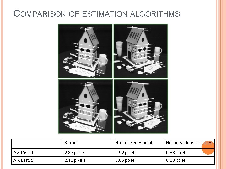
COMPARISON OF ESTIMATION ALGORITHMS 8 -point Normalized 8 -point Nonlinear least squares Av. Dist. 1 2. 33 pixels 0. 92 pixel 0. 86 pixel Av. Dist. 2 2. 18 pixels 0. 85 pixel 0. 80 pixel

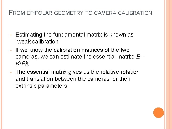
FROM EPIPOLAR GEOMETRY TO CAMERA CALIBRATION • • • Estimating the fundamental matrix is known as “weak calibration” If we know the calibration matrices of the two cameras, we can estimate the essential matrix: E = KTFK’ The essential matrix gives us the relative rotation and translation between the cameras, or their extrinsic parameters