CS 533 Modeling and Performance Evaluation of Network

CS 533 Modeling and Performance Evaluation of Network and Computer Systems Experimental Design (Chapters 16 -17) 1

Introduction (1 of 3) No experiment is ever a complete failure. It can always serve as a negative example. – Arthur Bloch The fundamental principle of science, the definition almost, is this: the sole test of the validity of any idea is experiment. – Richard P. Feynman • Goal is to obtain maximum information • • 2 with minimum number of experiments Proper analysis will help separate out the factors Statistical techniques will help determine if differences are caused by variations from errors or not

Introduction (2 of 3) • Key assumption is non-zero cost – Takes time and effort to gather data – Takes time and effort to analyze and draw conclusions Minimize number of experiments run • Good experimental design allows you to: – Isolate effects of each input variable – Determine effects due to interactions of input variables – Determine magnitude of experimental error – Obtain maximum info with minimum effort 3

Introduction (3 of 3) • Consider – Vary one input while holding others constant • Simple, but ignores possible interaction between two input variables – Test all possible combinations of input variables • Can determine interaction effects, but can be very large • Ex: 5 factors with 4 levels 45 = 1024 experiments. Repeating to get variation in measurement error 1024 x 3 = 3072 • There are, of course, in-between choices… – (Ch 19, but leads to confounding…) 4

Outline • Introduction • Terminology • General Mistakes • Simple Designs • Full Factorial Designs – 2 k Factorial Designs • 2 kr Factorial Designs 5

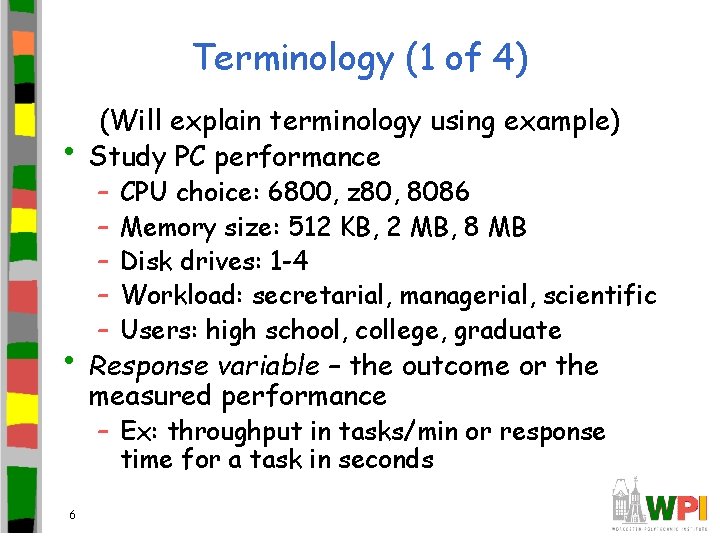
Terminology (1 of 4) • (Will explain terminology using example) Study PC performance – – – CPU choice: 6800, z 80, 8086 Memory size: 512 KB, 2 MB, 8 MB Disk drives: 1 -4 Workload: secretarial, managerial, scientific Users: high school, college, graduate • Response variable – the outcome or the measured performance – Ex: throughput in tasks/min or response time for a task in seconds 6

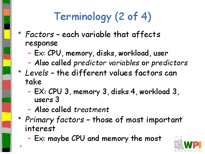
Terminology (2 of 4) • Factors – each variable that affects response – Ex: CPU, memory, disks, workload, user – Also called predictor variables or predictors • Levels – the different values factors can take – EX: CPU 3, memory 3, disks 4, workload 3, users 3 – Also called treatment • Primary factors – those of most important interest – Ex: maybe CPU and memory the most 7

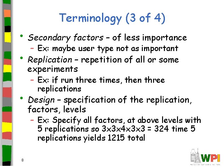
Terminology (3 of 4) • Secondary factors – of less importance – Ex: maybe user type not as important • Replication – repetition of all or some experiments – Ex: if run three times, then three replications • Design – specification of the replication, factors, levels – Ex: Specify all factors, at above levels with 5 replications so 3 x 3 x 4 x 3 x 3 = 324 time 5 replications yields 1215 total 8

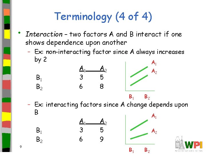
Terminology (4 of 4) • Interaction – two factors A and B interact if one shows dependence upon another – Ex: non-interacting factor since A always increases by 2 A 1 A 2 B 1 3 5 B 2 6 8 B 1 B 2 – Ex: interacting factors since A change depends upon B A 1 A 2 B 1 3 5 A 2 B 2 6 9 9

Outline • Introduction • Terminology • General Mistakes • Simple Designs • Full Factorial Designs – 2 k Factorial Designs • 2 kr Factorial Designs 10

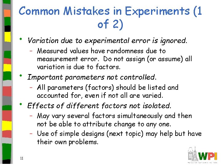
Common Mistakes in Experiments (1 of 2) • Variation due to experimental error is ignored. – Measured values have randomness due to measurement error. Do not assign (or assume) all variation is due to factors. • Important parameters not controlled. • Effects of different factors not isolated. 11 – All parameters (factors) should be listed and accounted for, even if not all are varied. – May vary several factors simultaneously and then not be able to attribute change to any one. – Use of simple designs (next topic) may help but have their own problems.

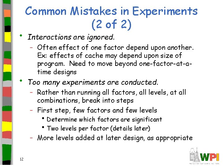
• • Common Mistakes in Experiments (2 of 2) Interactions are ignored. – Often effect of one factor depend upon another. Ex: effects of cache may depend upon size of program. Need to move beyond one-factor-at-atime designs Too many experiments are conducted. – Rather than running all factors, all levels, at all combinations, break into steps – First step, few factors and few levels • Determine which factors are significant • Two levels per factor (details later) – More levels added at later design, as appropriate 12

Outline • Introduction • Terminology • General Mistakes • Simple Designs • Full Factorial Designs – 2 k Factorial Designs • 2 kr Factorial Designs 13

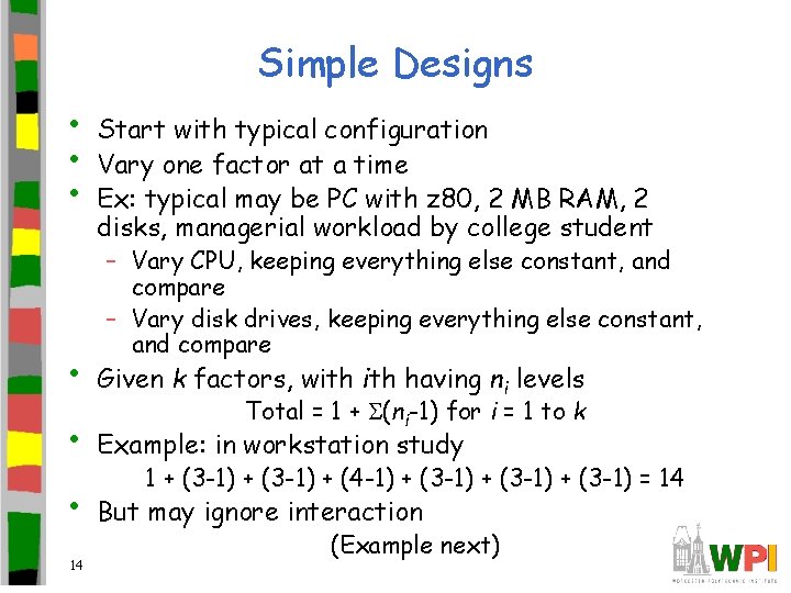
Simple Designs • • • Start with typical configuration Vary one factor at a time Ex: typical may be PC with z 80, 2 MB RAM, 2 disks, managerial workload by college student – Vary CPU, keeping everything else constant, and compare – Vary disk drives, keeping everything else constant, and compare • Given k factors, with having ni levels • Example: in workstation study • But may ignore interaction 14 Total = 1 + (ni-1) for i = 1 to k 1 + (3 -1) + (4 -1) + (3 -1) = 14 (Example next)

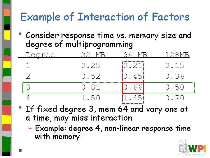
Example of Interaction of Factors • Consider response time vs. memory size and • degree of multiprogramming Degree 32 MB 64 MB 128 MB 1 0. 25 0. 21 0. 15 2 0. 52 0. 45 0. 36 3 0. 81 0. 66 0. 50 4 1. 50 1. 45 0. 70 If fixed degree 3, mem 64 and vary one at a time, may miss interaction – Example: degree 4, non-linear response time with memory 15

Outline • Introduction • Terminology • General Mistakes • Simple Designs • Full Factorial Designs – 2 k Factorial Designs • 2 kr Factorial Designs 16

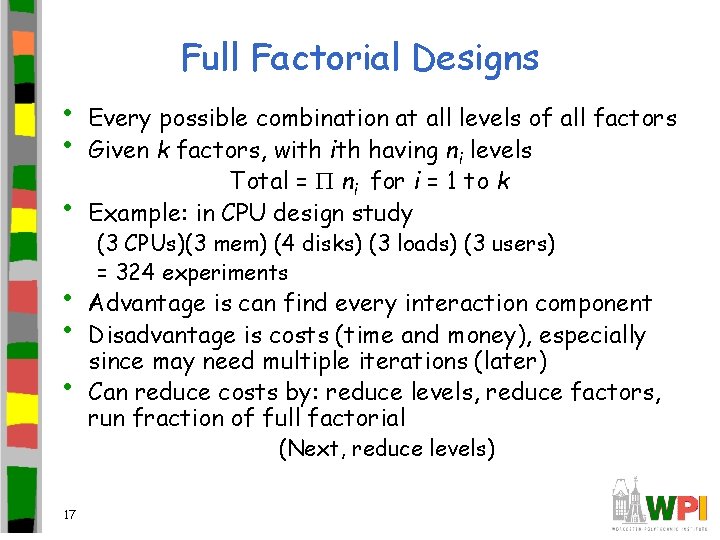
Full Factorial Designs • • • Every possible combination at all levels of all factors Given k factors, with having ni levels Total = ni for i = 1 to k Example: in CPU design study (3 CPUs)(3 mem) (4 disks) (3 loads) (3 users) = 324 experiments Advantage is can find every interaction component Disadvantage is costs (time and money), especially since may need multiple iterations (later) Can reduce costs by: reduce levels, reduce factors, run fraction of full factorial (Next, reduce levels) 17

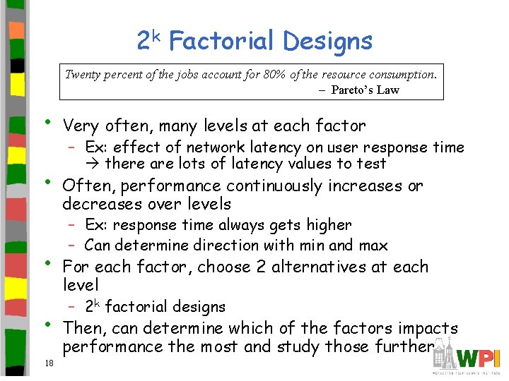
2 k Factorial Designs Twenty percent of the jobs account for 80% of the resource consumption. – Pareto’s Law • • 18 Very often, many levels at each factor – Ex: effect of network latency on user response time there are lots of latency values to test Often, performance continuously increases or decreases over levels – Ex: response time always gets higher – Can determine direction with min and max For each factor, choose 2 alternatives at each level – 2 k factorial designs Then, can determine which of the factors impacts performance the most and study those further

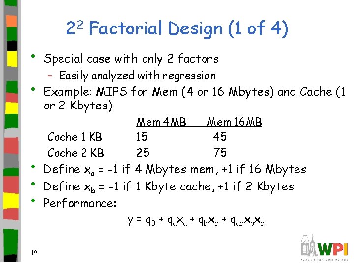
22 Factorial Design (1 of 4) • • • 19 Special case with only 2 factors – Easily analyzed with regression Example: MIPS for Mem (4 or 16 Mbytes) and Cache (1 or 2 Kbytes) Cache 1 KB Cache 2 KB Mem 4 MB 15 25 Mem 16 MB 45 75 Define xa = -1 if 4 Mbytes mem, +1 if 16 Mbytes Define xb = -1 if 1 Kbyte cache, +1 if 2 Kbytes Performance: y = q 0 + qaxa + qbxb + qabxaxb

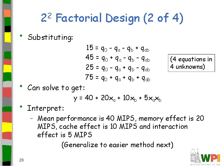
22 Factorial Design (2 of 4) • Substituting: • Can solve to get: • Interpret: 20 15 = q 0 - qa - qb + qab 45 = q 0 + qa - qb - qab 25 = q 0 - qa + qb - qab 75 = q 0 + qa + qb + qab (4 equations in 4 unknowns) y = 40 + 20 xa + 10 xb + 5 xaxb – Mean performance is 40 MIPS, memory effect is 20 MIPS, cache effect is 10 MIPS and interaction effect is 5 MIPS (Generalize to easier method next)

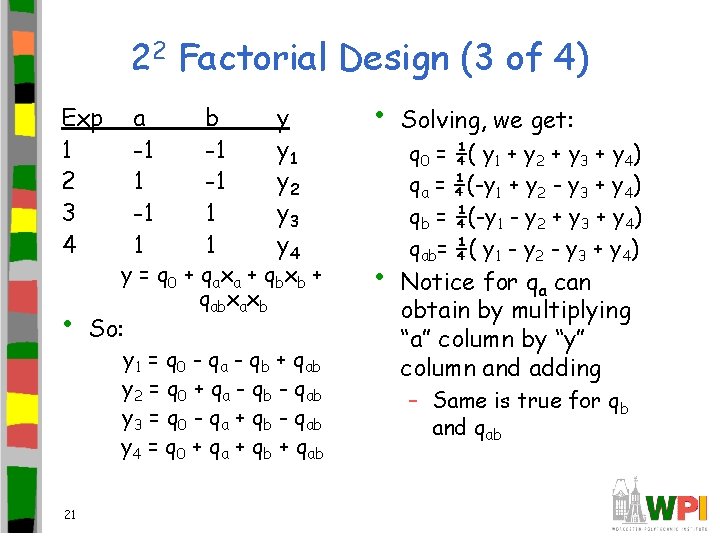
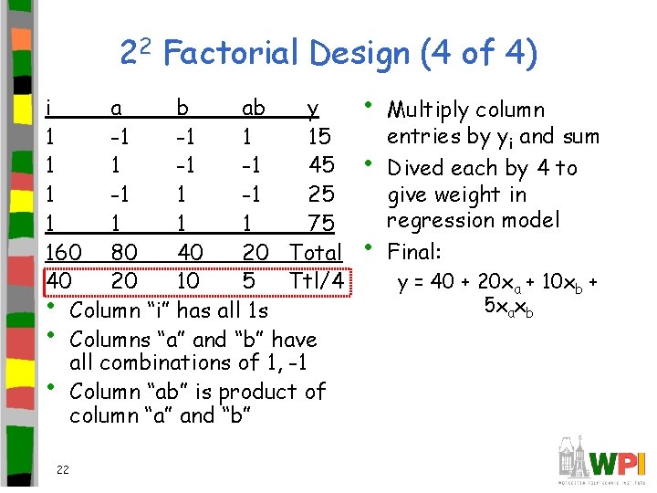
22 Factorial Design (3 of 4) Exp 1 2 3 4 • 21 a -1 1 b -1 -1 1 1 y y 1 y 2 y 3 y 4 y = q 0 + q a x a + q bx b + qabxaxb So: y 1 = q 0 - qa - qb + qab y 2 = q 0 + qa - qb - qab y 3 = q 0 - qa + qb - qab y 4 = q 0 + qa + qb + qab • • Solving, we get: q 0 = ¼( y 1 + y 2 + y 3 + y 4) qa = ¼(-y 1 + y 2 - y 3 + y 4) qb = ¼(-y 1 - y 2 + y 3 + y 4) qab= ¼( y 1 - y 2 - y 3 + y 4) Notice for qa can obtain by multiplying “a” column by “y” column and adding – Same is true for qb and qab

22 Factorial Design (4 of 4) i a b ab y 1 -1 -1 1 15 1 1 -1 -1 45 1 -1 25 1 1 75 160 80 40 20 Total 40 20 10 5 Ttl/4 • Column “i” has all 1 s • Columns “a” and “b” have all combinations of 1, -1 • Column “ab” is product of column “a” and “b” 22 • • • Multiply column entries by yi and sum Dived each by 4 to give weight in regression model Final: y = 40 + 20 xa + 10 xb + 5 xaxb

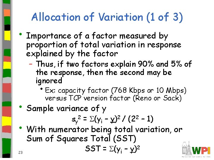
Allocation of Variation (1 of 3) • Importance of a factor measured by proportion of total variation in response explained by the factor – Thus, if two factors explain 90% and 5% of the response, then the second may be ignored • Ex: capacity factor (768 Kbps or 10 Mbps) versus TCP version factor (Reno or Sack) • Sample variance of y sy 2 = (yi – y)2 / (22 – 1) • With numerator being total variation, or Sum of Squares Total (SST) 23 SST = (yi – y)2

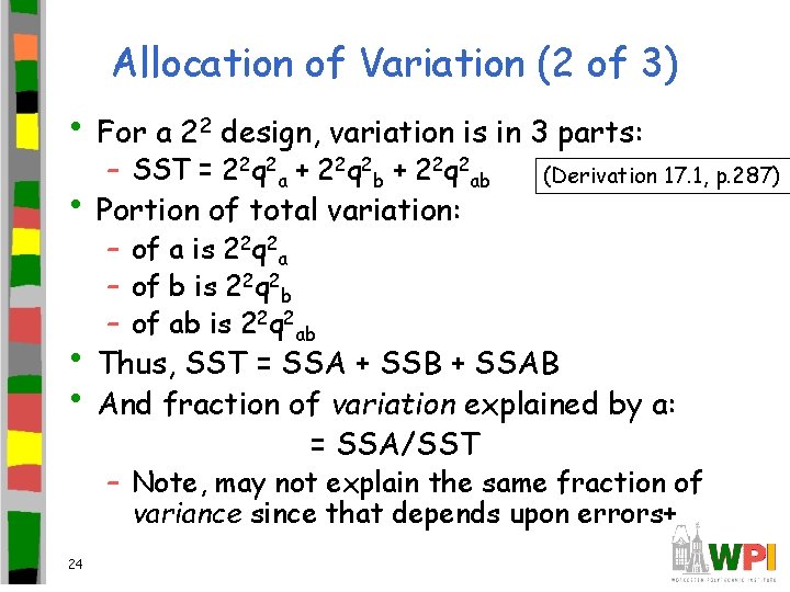
Allocation of Variation (2 of 3) • For a 22 design, variation is in 3 parts: – SST = 22 q 2 a + 22 q 2 b + 22 q 2 ab • Portion of total variation: (Derivation 17. 1, p. 287) – of a is 22 q 2 a – of b is 22 q 2 b – of ab is 22 q 2 ab • Thus, SST = SSA + SSB + SSAB • And fraction of variation explained by a: = SSA/SST – Note, may not explain the same fraction of variance since that depends upon errors+ 24

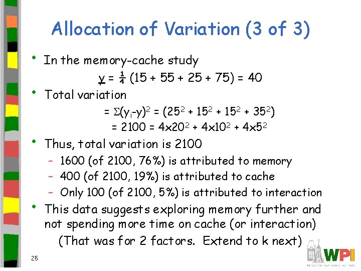
Allocation of Variation (3 of 3) • • In the memory-cache study y = ¼ (15 + 55 + 25 + 75) = 40 Total variation • Thus, total variation is 2100 • 25 = (yi-y)2 = (252 + 152 + 352) = 2100 = 4 x 202 + 4 x 102 + 4 x 52 – 1600 (of 2100, 76%) is attributed to memory – 400 (of 2100, 19%) is attributed to cache – Only 100 (of 2100, 5%) is attributed to interaction This data suggests exploring memory further and not spending more time on cache (or interaction) (That was for 2 factors. Extend to k next)

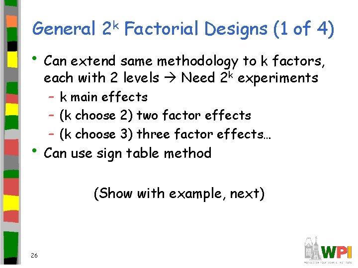
General 2 k Factorial Designs (1 of 4) • Can extend same methodology to k factors, each with 2 levels Need 2 k experiments – k main effects – (k choose 2) two factor effects – (k choose 3) three factor effects… • Can use sign table method (Show with example, next) 26

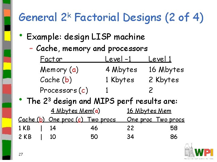
General 2 k Factorial Designs (2 of 4) • Example: design LISP machine – Cache, memory and processors Factor Memory (a) Cache (b) Processors (c) Level – 1 4 Mbytes 1 Kbytes 1 Level 1 16 Mbytes 2 Kbytes 2 • The 23 design and MIPS perf results are: 4 Mbytes Mem(a) Cache (b) One proc (c) Two procs 1 KB | 14 46 2 KB | 10 50 27 16 Mbytes Mem One proc Two procs 22 58 34 86

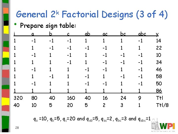
General 2 k Factorial Designs (3 of 4) • Prepare sign table: i 1 1 1 1 320 40 a -1 1 80 10 b -1 -1 1 1 40 5 c -1 -1 1 1 160 20 ab 1 -1 1 1 -1 -1 -1 1 40 5 ac 1 -1 -1 1 16 2 bc 1 1 -1 -1 1 1 24 3 abc -1 1 -1 -1 -1 1 9 1 qa =10, qb=5, qc=20 and qab=5, qac=2, qbc=3 and qabc=1 28 y 14 22 10 34 46 58 50 86 Ttl/8

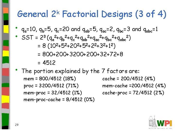
General 2 k Factorial Designs (3 of 4) • • • 29 qa=10, qb=5, qc=20 and qab=5, qac=2, qbc=3 and qabc=1 SST = 23 (qa 2+qb 2+qc 2+qab 2+qac 2+qbc 2+qabc 2) = 8 (102+52+22+32+12) = 800+200+32+72+8 = 4512 The portion explained by the 7 factors are: mem = 800/4512 (18%) proc = 3200/4512 (71%) mem-proc = 32/4512 (1%) mem-proc-cache = 8/4512 (0%) cache = 200/4512 (4%) mem-cache =200/4512 (4%) cache-proc = 72/4512 (2%)

Outline • Introduction • Terminology • General Mistakes • Simple Designs • Full Factorial Designs – 2 k Factorial Designs • 2 kr Factorial Designs 30

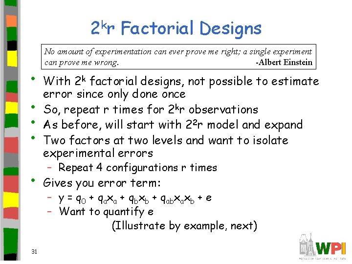
2 kr Factorial Designs • • • 31 No amount of experimentation can ever prove me right; a single experiment can prove me wrong. -Albert Einstein With 2 k factorial designs, not possible to estimate error since only done once So, repeat r times for 2 kr observations As before, will start with 22 r model and expand Two factors at two levels and want to isolate experimental errors – Repeat 4 configurations r times Gives you error term: – y = q 0 + qaxa + qbxb + qabxaxb + e – Want to quantify e (Illustrate by example, next)

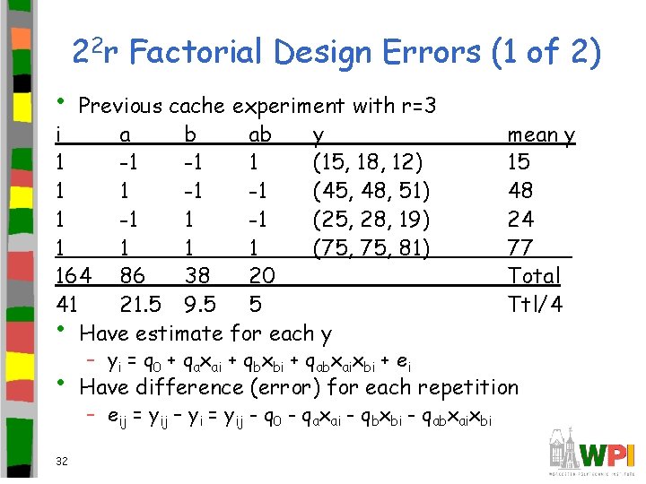
22 r Factorial Design Errors (1 of 2) • Previous cache experiment with r=3 i a b ab y 1 -1 -1 1 (15, 18, 12) 1 1 -1 -1 (45, 48, 51) 1 -1 (25, 28, 19) 1 1 (75, 81) 164 86 38 20 41 21. 5 9. 5 5 • Have estimate for each y • 32 – yi = q 0 + qaxai + qbxbi + qabxaixbi + ei mean y 15 48 24 77 Total Ttl/4 Have difference (error) for each repetition – eij = yij – yi = yij - q 0 - qaxai - qbxbi - qabxaixbi

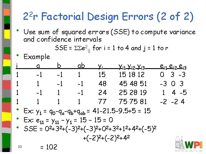
• • 22 r Factorial Design Errors (2 of 2) Use sum of squared errors (SSE) to compute variance and confidence intervals SSE = e 2 ij for i = 1 to 4 and j = 1 to r Example i a b ab yi yi 1 yi 2 yi 3 1 -1 -1 1 15 15 18 12 1 1 -1 -1 48 45 48 51 1 -1 24 25 28 19 1 1 77 75 75 81 • Ex: y 1 = q 0 -qa-qb+qab = 41 -21. 5 -9. 5+5 = 15 • Ex: e 11 = y 11 – y 1 = 15 – 15 = 0 • SSE = 02+32+(-3)2+02+32+12+42+(-5)2 +(-2)2+42 33 = 102 ei 1 ei 2 ei 3 0 3 -3 -3 0 3 1 4 -5 -2 -2 4

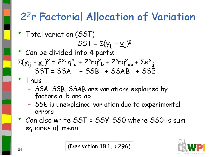
22 r Factorial Allocation of Variation • Total variation (SST) SST = (yij – y. . )2 • Can be divided into 4 parts: (yij – y. . )2 = 22 rq 2 a + 22 rq 2 b + 22 rq 2 ab + e 2 ij SST = SSA + SSB + SSAB + SSE • Thus • 34 – SSA, SSB, SSAB are variations explained by factors a, b and ab – SSE is unexplained variation due to experimental errors Can also write SST = SSY-SS 0 where SS 0 is sum squares of mean (Derivation 18. 1, p. 296)

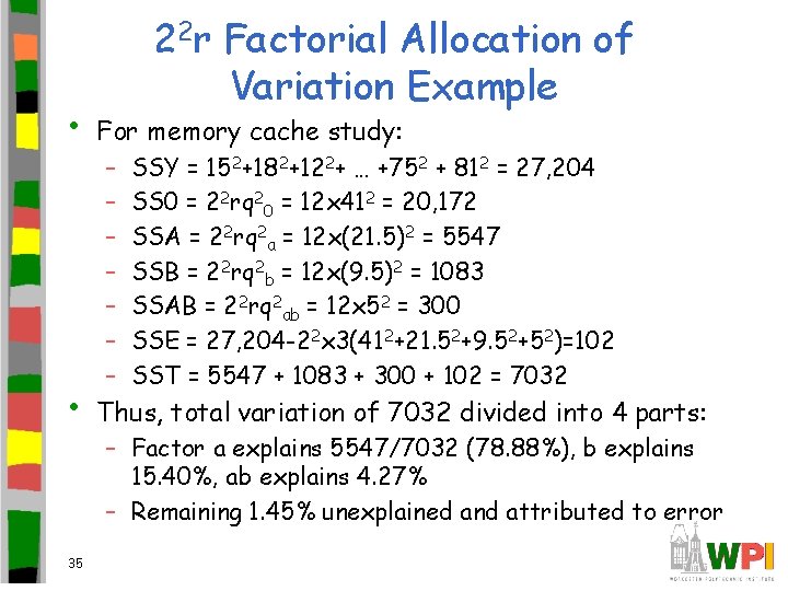
22 r Factorial Allocation of Variation Example • For memory cache study: • Thus, total variation of 7032 divided into 4 parts: 35 – – – – SSY = 152+182+122+ … +752 + 812 = 27, 204 SS 0 = 22 rq 20 = 12 x 412 = 20, 172 SSA = 22 rq 2 a = 12 x(21. 5)2 = 5547 SSB = 22 rq 2 b = 12 x(9. 5)2 = 1083 SSAB = 22 rq 2 ab = 12 x 52 = 300 SSE = 27, 204 -22 x 3(412+21. 52+9. 52+52)=102 SST = 5547 + 1083 + 300 + 102 = 7032 – Factor a explains 5547/7032 (78. 88%), b explains 15. 40%, ab explains 4. 27% – Remaining 1. 45% unexplained and attributed to error

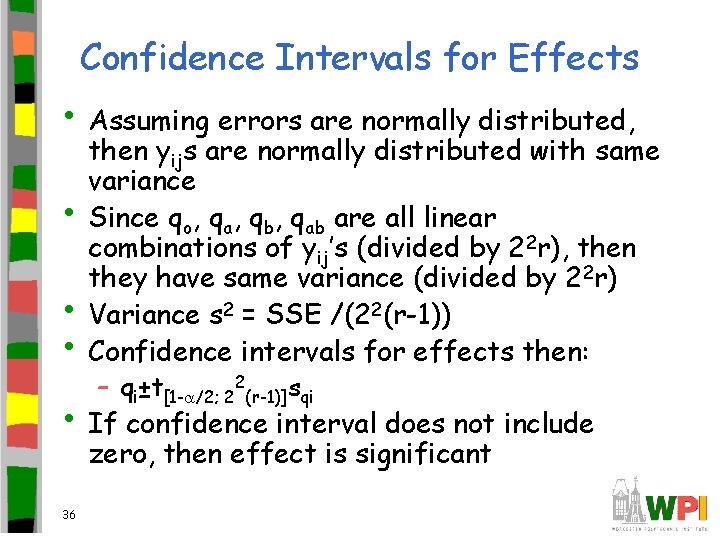
Confidence Intervals for Effects • Assuming errors are normally distributed, • • • then yijs are normally distributed with same variance Since qo, qa, qb, qab are all linear combinations of yij’s (divided by 22 r), then they have same variance (divided by 22 r) Variance s 2 = SSE /(22(r-1)) Confidence intervals for effects then: – qi±t[1 - /2; 22(r-1)]sqi • If confidence interval does not include zero, then effect is significant 36

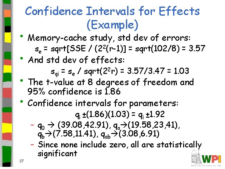
Confidence Intervals for Effects (Example) • Memory-cache study, std dev of errors: se = sqrt[SSE / (22(r-1)] = sqrt(102/8) = 3. 57 • And std dev of effects: sqi = se / sqrt(22 r) = 3. 57/3. 47 = 1. 03 • The t-value at 8 degrees of freedom and • 37 95% confidence is 1. 86 Confidence intervals for parameters: qi ±(1. 86)(1. 03) = qi ± 1. 92 – q 0 (39. 08, 42. 91), qa (19. 58, 23, 41), qb (7. 58, 11. 41), qab (3. 08, 6. 91) – Since none include zero, all are statistically significant

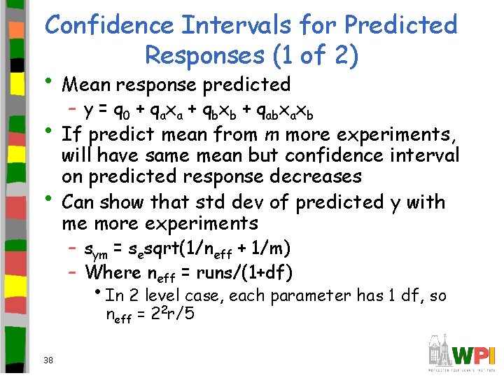
Confidence Intervals for Predicted Responses (1 of 2) • Mean response predicted – y = q 0 + qaxa + qbxb + qabxaxb • If predict mean from m more experiments, • will have same mean but confidence interval on predicted response decreases Can show that std dev of predicted y with me more experiments – sym = sesqrt(1/neff + 1/m) – Where neff = runs/(1+df) • In 2 level case, each parameter has 1 df, so neff = 22 r/5 38

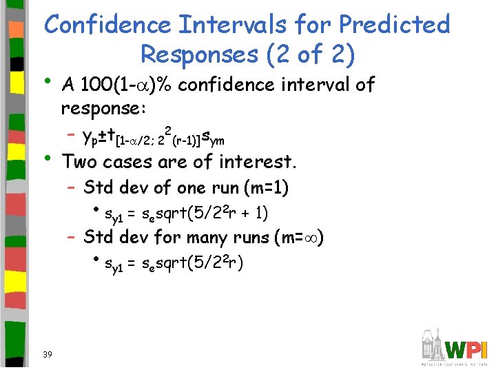
Confidence Intervals for Predicted Responses (2 of 2) • A 100(1 - )% confidence interval of response: – yp±t[1 - /2; 22(r-1)]sym • Two cases are of interest. – Std dev of one run (m=1) • sy 1 = sesqrt(5/22 r + 1) – Std dev for many runs (m= ) • sy 1 = sesqrt(5/22 r) 39

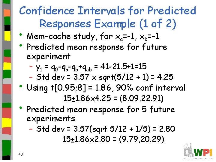
Confidence Intervals for Predicted Responses Example (1 of 2) • Mem-cache study, for xa=-1, xb=-1 • Predicted mean response for future experiment – y 1 = q 0 -qa-qb+qab = 41 -21. 5+1=15 – Std dev = 3. 57 x sqrt(5/12 + 1) = 4. 25 • Using t[0. 95; 8] = 1. 86, 90% conf interval 15± 1. 86 x 4. 25 = (8. 09, 22. 91) • Predicted mean response for 5 future experiments – Std dev = 3. 57(sqrt 5/12 + 1/5) = 2. 80 15± 1. 86 x 2. 80 = (9. 79, 20. 29) 40

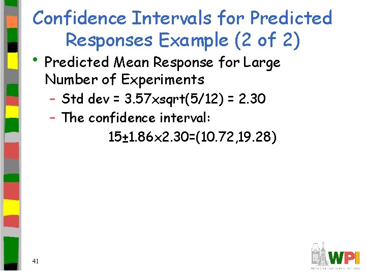
Confidence Intervals for Predicted Responses Example (2 of 2) • Predicted Mean Response for Large Number of Experiments – Std dev = 3. 57 xsqrt(5/12) = 2. 30 – The confidence interval: 15± 1. 86 x 2. 30=(10. 72, 19. 28) 41