CS 5263 CS 4593 Bioinformatics Exact String Matching

CS 5263 & CS 4593 Bioinformatics Exact String Matching Algorithms

Overview • Sequence alignment: two sub-problems: – How to score an alignment with errors – How to find an alignment with the best score • Today: exact string matching – Does not allow any errors – Efficiency becomes the sole consideration • Time and space

Why exact string matching? • The most fundamental string comparison problem • Often the core of more complex string comparison algorithms – E. g. , BLAST • Often repeatedly called by other methods – Usually the most time consuming part – Small improvement could improve overall efficiency considerably

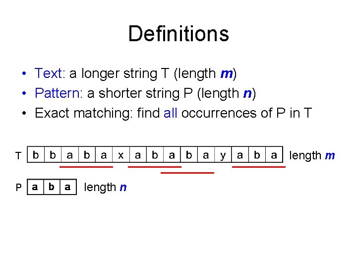
Definitions • Text: a longer string T (length m) • Pattern: a shorter string P (length n) • Exact matching: find all occurrences of P in T length m T P length n

The naïve algorithm

Time complexity • Worst case: O(mn) • How to speedup? – Pre-processing T or P – Why pre-processing can save us time? • Uncovers the structure of T or P • Determines when we can skip ahead without missing anything • Determines when we can infer the result of character comparisons without doing them.

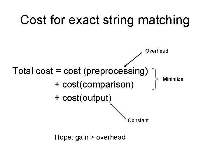
Cost for exact string matching Overhead Total cost = cost (preprocessing) + cost(comparison) + cost(output) Constant Hope: gain > overhead Minimize

String matching scenarios • One T and one P – Search a word in a document • One T and many P all at once – Search a set of words in a document – Spell checking (fixed P) • One fixed T, many P – Search a completed genome for short sequences • Two (or many) T’s for common patterns • Q: Which one to pre-process? • A: Always pre-process the shorter seq, or the one that is repeatedly used

Pre-processing algs • Pattern preprocessing – Knuth-Morris-Pratt algorithm (KMP) – Aho-Corasick algorithm • Multiple patterns – Boyer – Moore algorithm (discuss if have time) • The choice of most cases • Typically sub-linear time • Text preprocessing – Suffix tree • Very useful for many purposes – Suffix array – Burrows-Wheeler Transformation

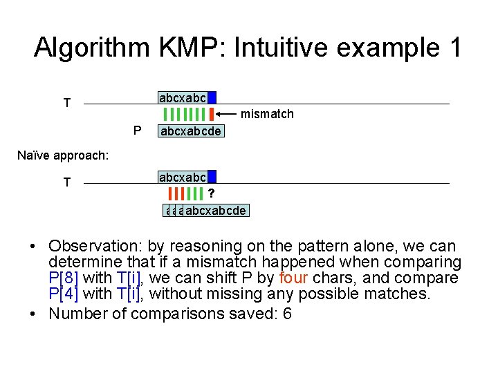
Algorithm KMP: Intuitive example 1 abcxabc T mismatch P abcxabcde Naïve approach: T abcxabc ? abcxabcde • Observation: by reasoning on the pattern alone, we can determine that if a mismatch happened when comparing P[8] with T[i], we can shift P by four chars, and compare P[4] with T[i], without missing any possible matches. • Number of comparisons saved: 6

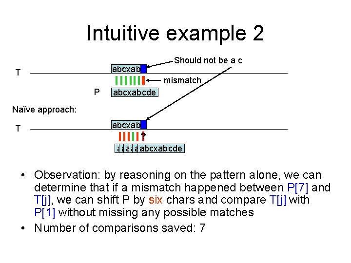
Intuitive example 2 abcxabc T Should not be a c mismatch P abcxabcde Naïve approach: T abcxabc ? abcxabcde abcxabcde • Observation: by reasoning on the pattern alone, we can determine that if a mismatch happened between P[7] and T[j], we can shift P by six chars and compare T[j] with P[1] without missing any possible matches • Number of comparisons saved: 7

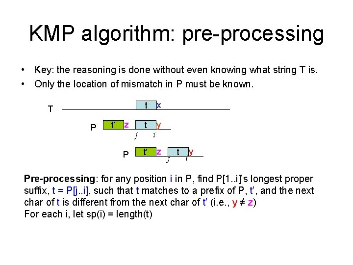
KMP algorithm: pre-processing • Key: the reasoning is done without even knowing what string T is. • Only the location of mismatch in P must be known. T P t’ z P j t x t y t’ i z j t i y Pre-processing: for any position i in P, find P[1. . i]’s longest proper suffix, t = P[j. . i], such that t matches to a prefix of P, t’, and the next char of t is different from the next char of t’ (i. e. , y ≠ z) For each i, let sp(i) = length(t)

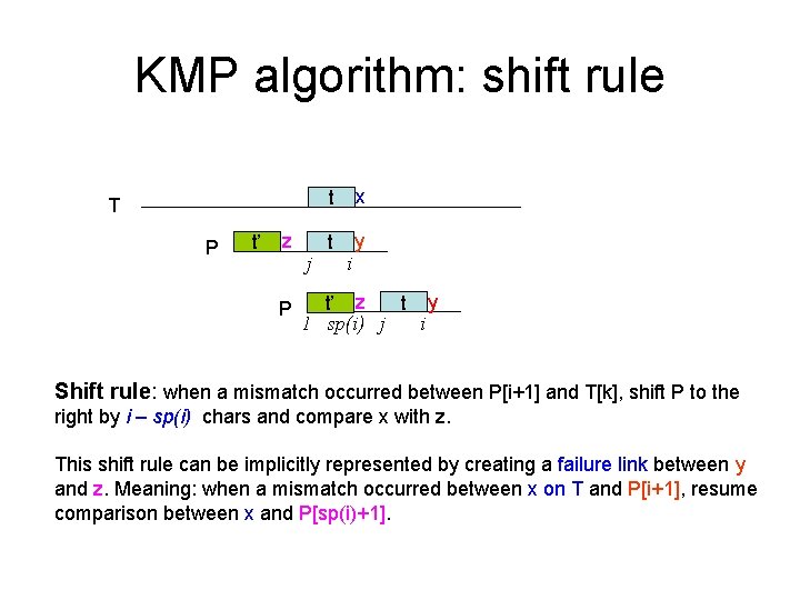
KMP algorithm: shift rule T P t’ z P j t x t y i t y t’ z 1 sp(i) j i Shift rule: when a mismatch occurred between P[i+1] and T[k], shift P to the right by i – sp(i) chars and compare x with z. This shift rule can be implicitly represented by creating a failure link between y and z. Meaning: when a mismatch occurred between x on T and P[i+1], resume comparison between x and P[sp(i)+1].

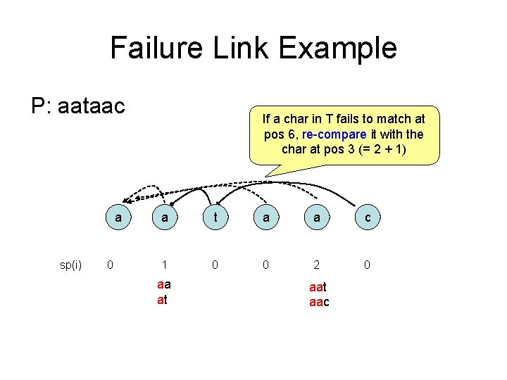
Failure Link Example P: aataac a sp(i) 0 If a char in T fails to match at pos 6, re-compare it with the char at pos 3 (= 2 + 1) a t a a c 1 0 0 2 0 aa at aac

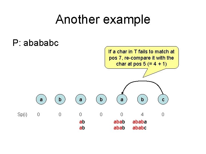
Another example P: abababc If a char in T fails to match at pos 7, re-compare it with the char at pos 5 (= 4 + 1) a Sp(i) 0 b a b c 0 0 4 0 ab ab ababa ababc

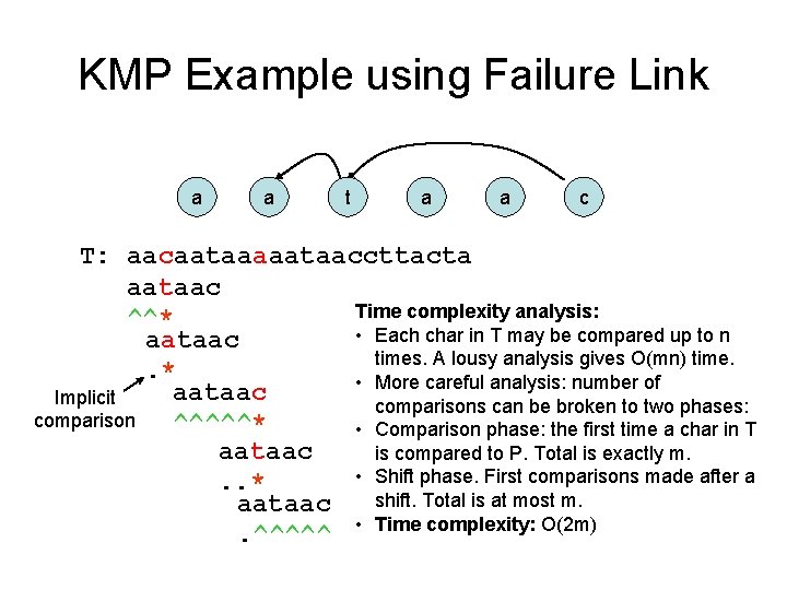
KMP Example using Failure Link a a t a a c T: aacaataaaaataaccttacta aataac Time complexity analysis: ^^* • Each char in T may be compared up to n aataac times. A lousy analysis gives O(mn) time. . * • More careful analysis: number of aataac Implicit comparisons can be broken to two phases: comparison ^^^^^* • Comparison phase: the first time a char in T aataac is compared to P. Total is exactly m. • Shift phase. First comparisons made after a. . * shift. Total is at most m. aataac. ^^^^^ • Time complexity: O(2 m)

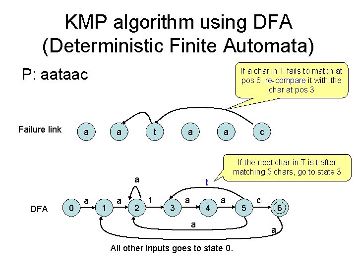
KMP algorithm using DFA (Deterministic Finite Automata) P: aataac Failure link If a char in T fails to match at pos 6, re-compare it with the char at pos 3 a a t a DFA 0 1 a 2 c If the next char in T is t after matching 5 chars, go to state 3 a a a t t 3 a 4 a a All other inputs goes to state 0. 5 c 6 a

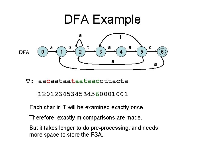
DFA Example a DFA 0 a 1 a 2 t t 3 a 4 a 5 a c 6 a T: aacaataataataaccttacta 1201234534534560001001 Each char in T will be examined exactly once. Therefore, exactly m comparisons are made. But it takes longer to do pre-processing, and needs more space to store the FSA.

Difference between Failure Link and DFA • Failure link – Preprocessing time and space are O(n), regardless of alphabet size – Comparison time is at most 2 m (at least m) • DFA – Preprocessing time and space are O(n | |) • May be a problem for very large alphabet size • For example, each “char” is a big integer • Chinese characters – Comparison time is always m.

The set matching problem • Find all occurrences of a set of patterns in T • First idea: run KMP or BM for each P – O(km + n) • k: number of patterns • m: length of text • n: total length of patterns • Better idea: combine all patterns together and search in one run

A simpler problem: spell-checking • A dictionary contains five words: – – – potato poetry pottery science school • Given a document, check if any word is (not) in the dictionary – Words in document are separated by special chars. – Relatively easy.

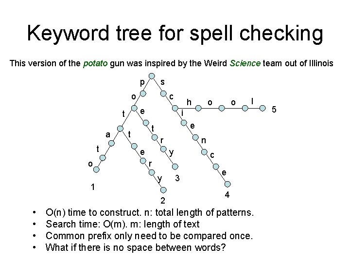
Keyword tree for spell checking This version of the potato gun was inspired by the Weird Science team out of Illinois p s o t o 1 o o l i e t t r e n y c r y 2 • • h e t a c 3 e 4 O(n) time to construct. n: total length of patterns. Search time: O(m). m: length of text Common prefix only need to be compared once. What if there is no space between words? 5

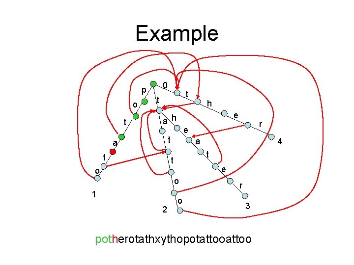
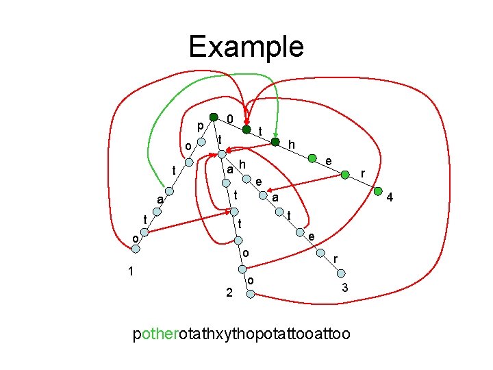
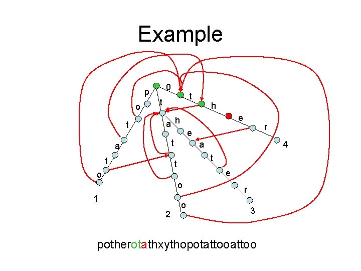
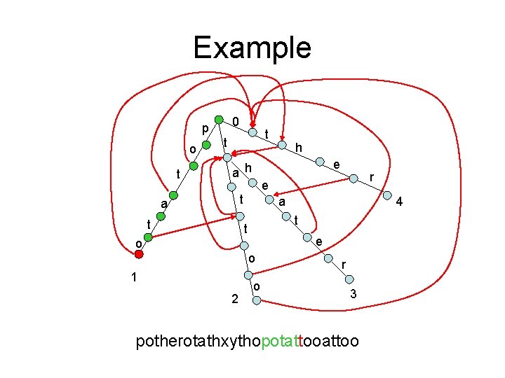
Aho-Corasick algorithm • Basis of the fgrep algorithm • Generalizing KMP – Using failure links • Example: given the following 4 patterns: – potato – tattoo – theater – other

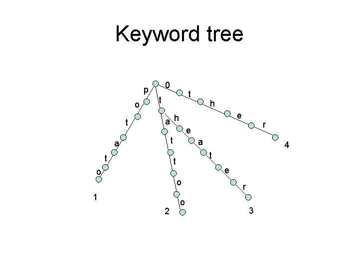
Keyword tree 0 p o t t t e a h t a e o o 2 4 t t 1 r e t a h o r 3

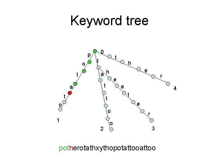
Keyword tree 0 p o t t t e a h t a e o o 2 4 t t 1 r e t a h o r 3 potherotathxythopotattoo

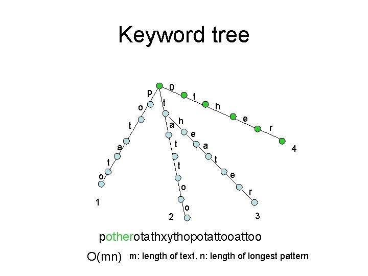
Keyword tree 0 p o t t t e a h t a e o o 2 4 t t 1 r e t a h o r 3 potherotathxythopotattoo O(mn) m: length of text. n: length of longest pattern

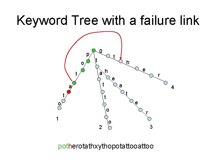
Keyword Tree with a failure link 0 p o t t t e a h t a e o o 2 4 t t 1 r e t a h o r 3 potherotathxythopotattoo

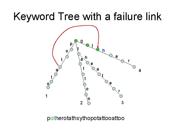
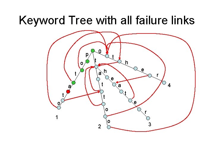
Keyword Tree with all failure links 0 p o t t t e a h t a e o o 2 4 t t 1 r e t a h o r 3

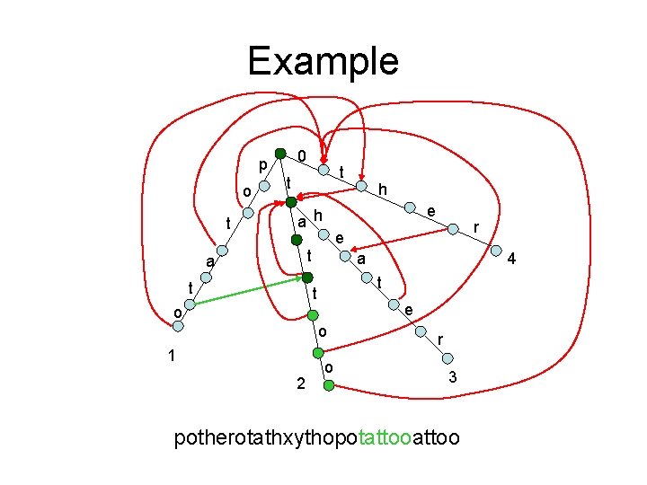
Example 0 p o t t t e a h t a e o o 2 4 t t 1 r e t a h o r 3 potherotathxythopotattoo

Aho-Corasick algorithm • O(n) preprocessing, and O(m+k) searching. – n: total length of patterns. – m: length of text – k is # of occurrence.

Suffix Tree • All algorithms we talked about so far preprocess pattern(s) – Boyer-Moore: fastest in practice. O(m) worst case. – KMP: O(m) – Aho-Corasick: O(m) • In some cases we may prefer to pre-process T – Fixed T, varying P • Suffix tree: basically a keyword tree of all suffixes

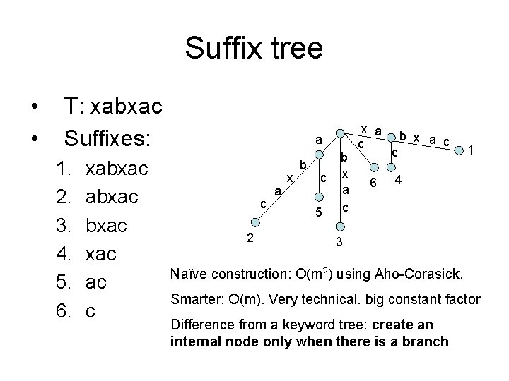
Suffix tree • • T: xabxac Suffixes: 1. 2. 3. 4. 5. 6. xabxac ac c a c 2 a x b c 5 b x a c 6 c b x a c 1 4 3 Naïve construction: O(m 2) using Aho-Corasick. Smarter: O(m). Very technical. big constant factor Difference from a keyword tree: create an internal node only when there is a branch

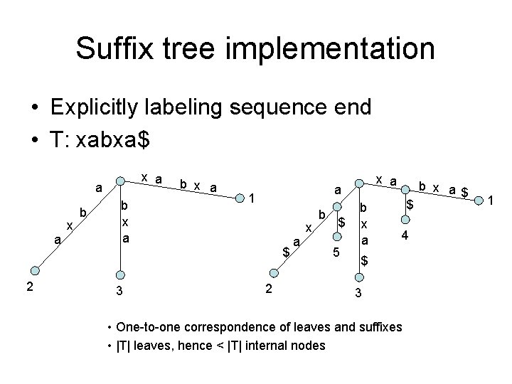
Suffix tree implementation • Explicitly labeling sequence end • T: xabxa$ x a a a 2 x b b x a a 1 $ 3 x a 2 a x b $ 5 b x a $ 4 $ 3 • One-to-one correspondence of leaves and suffixes • |T| leaves, hence < |T| internal nodes b x a$ 1

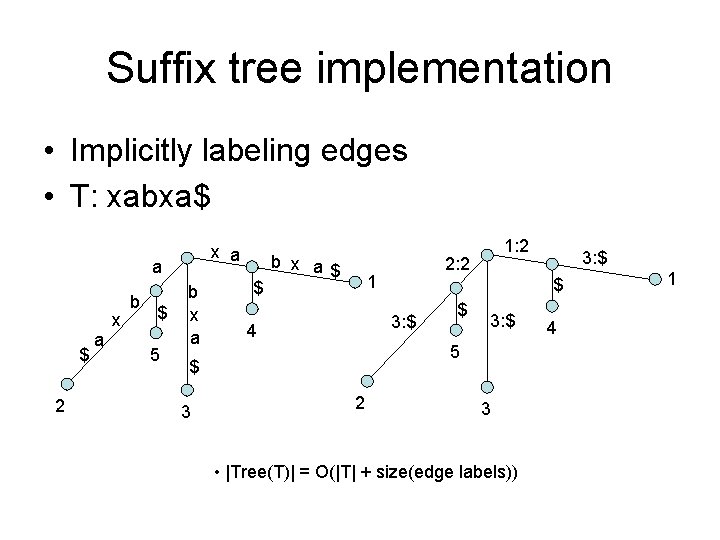
Suffix tree implementation • Implicitly labeling edges • T: xabxa$ x a a $ 2 a x b $ 5 b x a $ b x a$ $ 3: $ 5 2 3: $ $ 3 2: 2 1 4 1: 2 3 • |Tree(T)| = O(|T| + size(edge labels)) 4 1

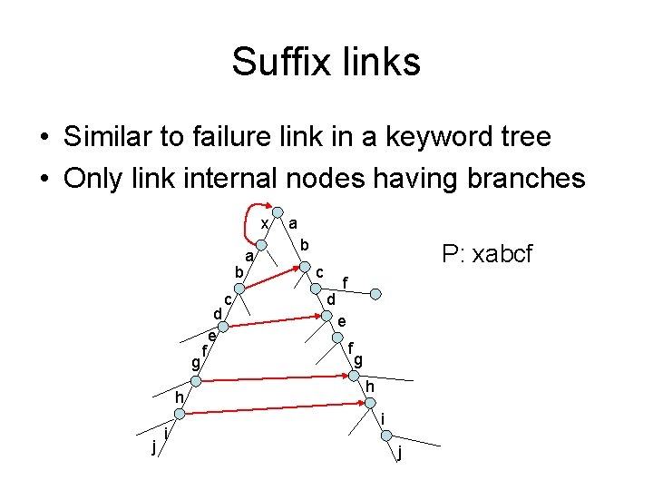
Suffix links • Similar to failure link in a keyword tree • Only link internal nodes having branches x b g h j i f d e c a a b P: xabcf c d f e f g h i j

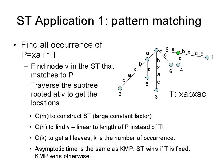
ST Application 1: pattern matching • Find all occurrence of P=xa in T – Find node v in the ST that matches to P – Traverse the subtree rooted at v to get the locations a c a x b c 5 2 b x a c 3 x a c 6 c b x a c 4 T: xabxac • O(m) to construct ST (large constant factor) • O(n) to find v – linear to length of P instead of T! • O(k) to get all leaves, k is the number of occurrence. • Asymptotic time is the same as KMP. ST wins if T is fixed. KMP wins otherwise. 1

ST application 2: repeats finding • Genome contains many repeated DNA sequences • Repeat sequence length: Varies from 1 nucleotide to millions – Genes may have multiple copies (50 to 10, 000) – Highly repetitive DNA in some non-coding regions • 6 to 10 bp x 100, 000 to 1, 000 times • Problem: find all repeats that are at least kresidues long and appear at least p times in the genome

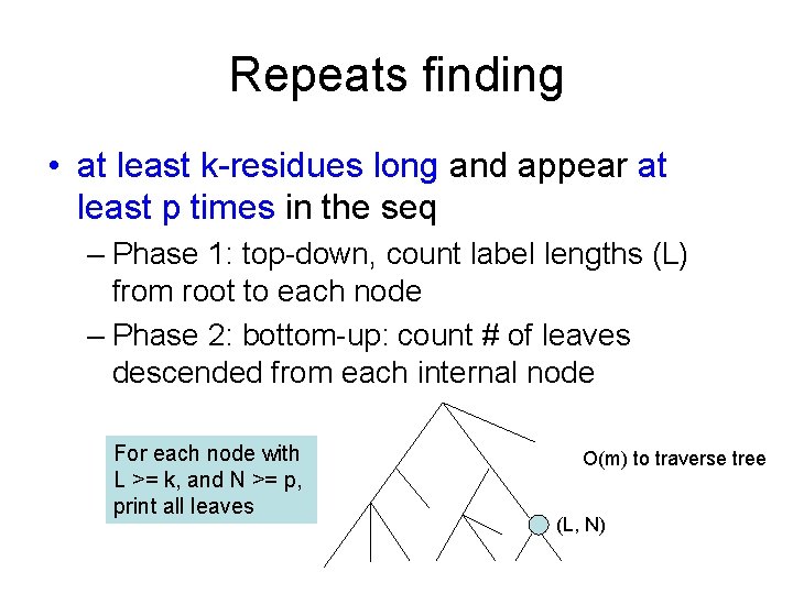
Repeats finding • at least k-residues long and appear at least p times in the seq – Phase 1: top-down, count label lengths (L) from root to each node – Phase 2: bottom-up: count # of leaves descended from each internal node For each node with L >= k, and N >= p, print all leaves O(m) to traverse tree (L, N)

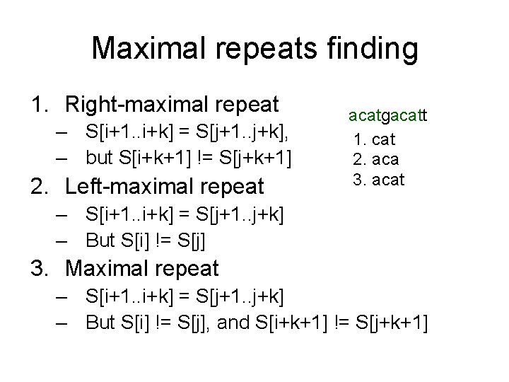
Maximal repeats finding 1. Right-maximal repeat – S[i+1. . i+k] = S[j+1. . j+k], – but S[i+k+1] != S[j+k+1] 2. Left-maximal repeat acatgacatt 1. cat 2. aca 3. acat – S[i+1. . i+k] = S[j+1. . j+k] – But S[i] != S[j] 3. Maximal repeat – S[i+1. . i+k] = S[j+1. . j+k] – But S[i] != S[j], and S[i+k+1] != S[j+k+1]

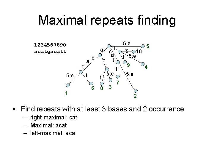
Maximal repeats finding 1234567890 acatgacatt a t 5: e 1 a c t t 6 8 5: e 5 $ 10 t 5: e t c a t t 5: e 3 t 9 4 5: e 7 2 • Find repeats with at least 3 bases and 2 occurrence – right-maximal: cat – Maximal: acat – left-maximal: aca

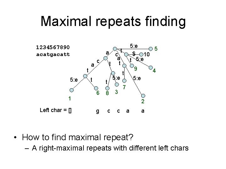
Maximal repeats finding 1234567890 acatgacatt a t 5: e 1 Left char = [] a c t c a t t t 6 5: e 5 $ 10 t 5: e t 8 5: e 3 9 t 4 5: e 7 2 g c c a a • How to find maximal repeat? – A right-maximal repeats with different left chars

Joint Suffix Tree (JST) • • • Build a ST for more than two strings Two strings S 1 and S 2 S* = S 1 & S 2 Build a suffix tree for S* in time O(|S 1| + |S 2|) The separator will only appear in the edge ending in a leaf (why? )

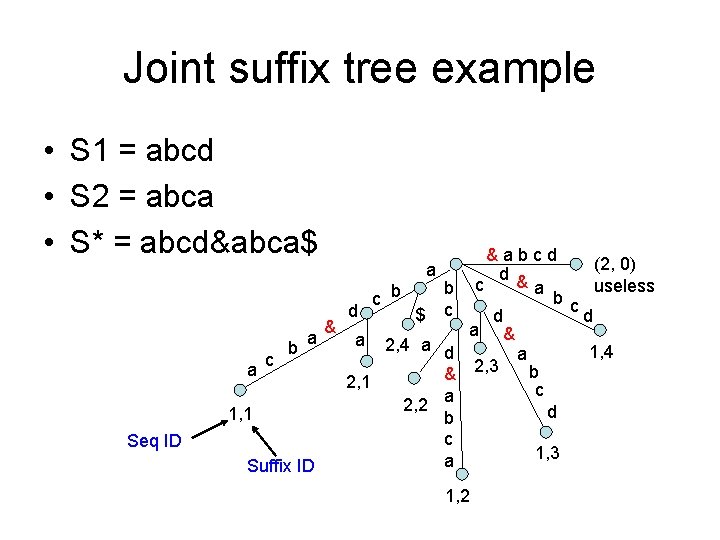
Joint suffix tree example • S 1 = abcd • S 2 = abca • S* = abcd&abca$ a c b a 1, 1 Seq ID Suffix ID a & d a c b $ b c 2, 4 a d & 2, 1 a 2, 2 b c a &abcd (2, 0) d & c useless a b c d d a & 1, 4 a 2, 3 b c d 1, 2 1, 3

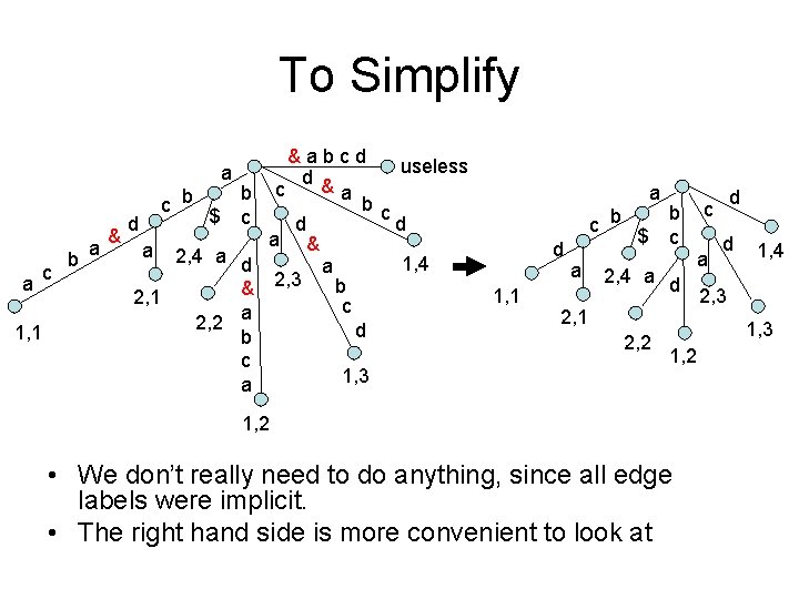
To Simplify a a 1, 1 c b a & c b d a $ b c 2, 4 a d & 2, 1 a 2, 2 b c a &abcd useless d & c a b c d d a & 1, 4 a 2, 3 b c d 1, 3 a c b d 1, 1 a $ b c 2, 4 a d 2, 1 2, 2 d c a d 1, 4 2, 3 1, 2 • We don’t really need to do anything, since all edge labels were implicit. • The right hand side is more convenient to look at

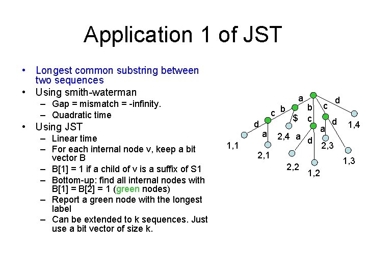
Application 1 of JST • Longest common substring between two sequences • Using smith-waterman a – Gap = mismatch = -infinity. – Quadratic time c b d • Using JST – Linear time – For each internal node v, keep a bit vector B – B[1] = 1 if a child of v is a suffix of S 1 – Bottom-up: find all internal nodes with B[1] = B[2] = 1 (green nodes) – Report a green node with the longest label – Can be extended to k sequences. Just use a bit vector of size k. 1, 1 a $ b c 2, 4 a d 2, 1 2, 2 d c a d 1, 4 2, 3 1, 2

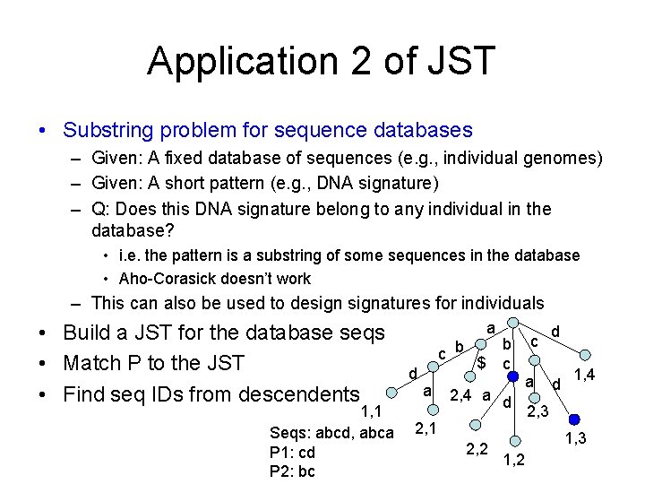
Application 2 of JST • Substring problem for sequence databases – Given: A fixed database of sequences (e. g. , individual genomes) – Given: A short pattern (e. g. , DNA signature) – Q: Does this DNA signature belong to any individual in the database? • i. e. the pattern is a substring of some sequences in the database • Aho-Corasick doesn’t work – This can also be used to designatures for individuals • Build a JST for the database seqs • Match P to the JST • Find seq IDs from descendents 1, 1 Seqs: abcd, abca P 1: cd P 2: bc a c b d a $ b c 2, 4 a d 2, 1 2, 2 c a d d 1, 4 2, 3 1, 2

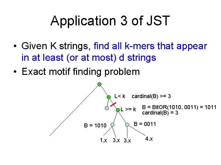
Application 3 of JST • Given K strings, find all k-mers that appear in at least (or at most) d strings • Exact motif finding problem L< k cardinal(B) >= 3 L >= k B = 0011 B = 1010 1, x B = Bit. OR(1010, 0011) = 1011 cardinal(B) = 3 3, x 4, x

Combinatorial motif finding • Idea 1: find all k-mers that appeared at least m times – m may be chosen such that # occurrence is statistically significant – Problem: most motifs have divergence. Each variation may only appear once. • Idea 2: find all k-mers, considering IUPAC nucleic acid codes – e. g. ASGTKTKAC, S = C/G, K = G/T – Still inflexible • Idea 3: find k-mers that approximately appeared at least m times – i. e. allow some mismatches

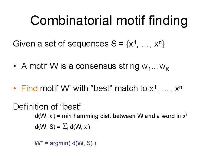
Combinatorial motif finding Given a set of sequences S = {x 1, …, xn} • A motif W is a consensus string w 1…w. K • Find motif W* with “best” match to x 1, …, xn Definition of “best”: d(W, xi) = min hamming dist. between W and a word in xi d(W, S) = i d(W, xi) W* = argmin( d(W, S) )

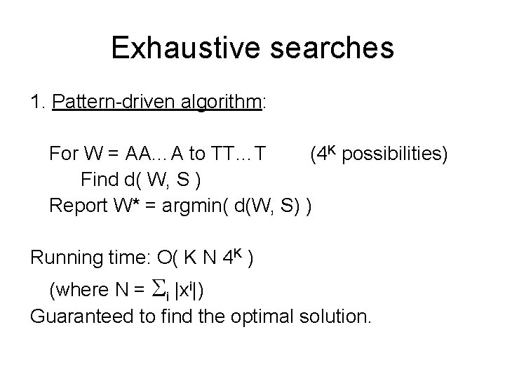
Exhaustive searches 1. Pattern-driven algorithm: For W = AA…A to TT…T (4 K possibilities) Find d( W, S ) Report W* = argmin( d(W, S) ) Running time: O( K N 4 K ) (where N = i |xi|) Guaranteed to find the optimal solution.

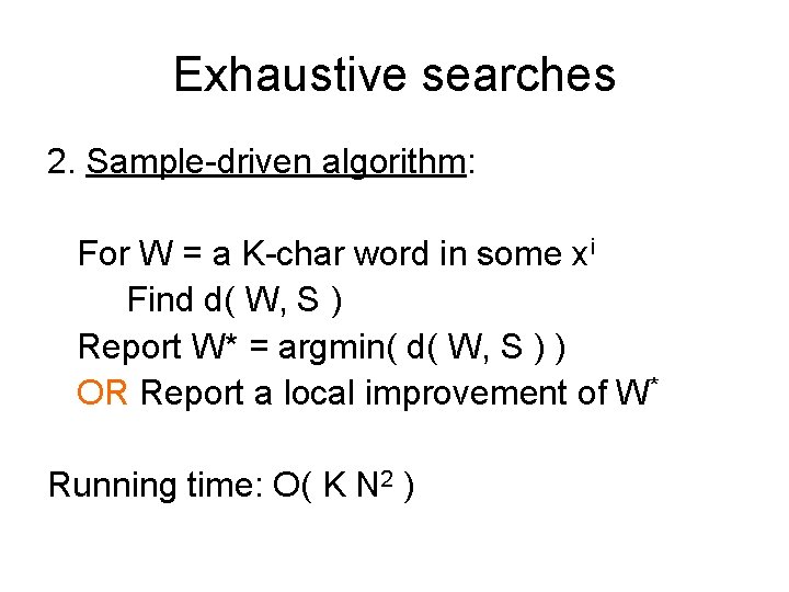
Exhaustive searches 2. Sample-driven algorithm: For W = a K-char word in some xi Find d( W, S ) Report W* = argmin( d( W, S ) ) OR Report a local improvement of W* Running time: O( K N 2 )

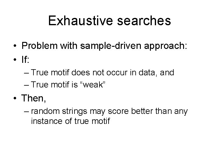
Exhaustive searches • Problem with sample-driven approach: • If: – True motif does not occur in data, and – True motif is “weak” • Then, – random strings may score better than any instance of true motif

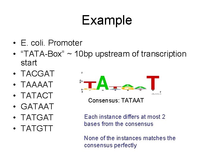
Example • E. coli. Promoter • “TATA-Box” ~ 10 bp upstream of transcription start • TACGAT • TAAAAT • TATACT Consensus: TATAAT • GATAAT Each instance differs at most 2 • TATGAT bases from the consensus • TATGTT None of the instances matches the consensus perfectly

Heuristic methods • Cannot afford exhaustive search on all patterns • Sample-driven approaches may miss real patterns • However, a real pattern should not differ too much from its instances in S • Start from the space of all words in S, extend to the space with real patterns

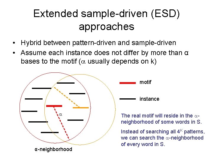
Extended sample-driven (ESD) approaches • Hybrid between pattern-driven and sample-driven • Assume each instance does not differ by more than α bases to the motif ( usually depends on k) motif instance α-neighborhood The real motif will reside in the neighborhood of some words in S. Instead of searching all 4 K patterns, we can search the -neighborhood of every word in S.

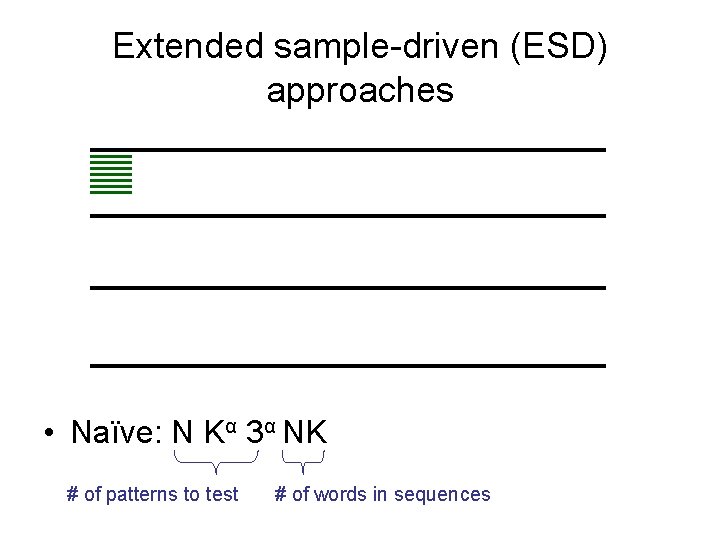
Extended sample-driven (ESD) approaches • Naïve: N Kα 3α NK # of patterns to test # of words in sequences

Better idea • Using a joint suffix tree, find all patterns that: – Have length K – Appeared in at least m sequences with at most α mismatches • Post-processing

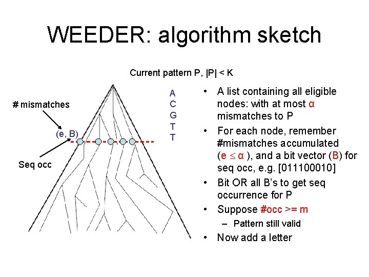
WEEDER: algorithm sketch Current pattern P, |P| < K # mismatches (e, B) Seq occ A C G T T • A list containing all eligible nodes: with at most α mismatches to P • For each node, remember #mismatches accumulated (e α ), and a bit vector (B) for seq occ, e. g. [011100010] • Bit OR all B’s to get seq occurrence for P • Suppose #occ >= m – Pattern still valid • Now add a letter

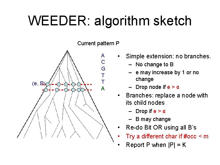
WEEDER: algorithm sketch Current pattern P (e, B) A C G T T A • Simple extension: no branches. – No change to B – e may increase by 1 or no change – Drop node if e > α • Branches: replace a node with its child nodes – Drop if e > α – B may change • Re-do Bit OR using all B’s • Try a different char if #occ < m • Report P when |P| = K

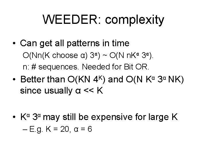
WEEDER: complexity • Can get all patterns in time O(Nn(K choose α) 3α) ~ O(N n. Kα 3α). n: # sequences. Needed for Bit OR. • Better than O(KN 4 K) and O(N Kα 3α NK) since usually α << K • Kα 3α may still be expensive for large K – E. g. K = 20, α = 6

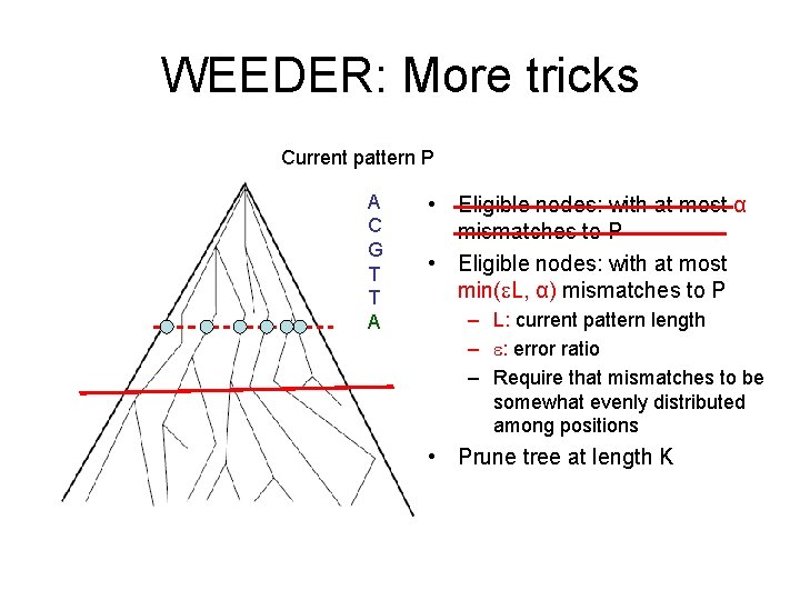
WEEDER: More tricks Current pattern P A C G T T A • Eligible nodes: with at most α mismatches to P • Eligible nodes: with at most min( L, α) mismatches to P – L: current pattern length – : error ratio – Require that mismatches to be somewhat evenly distributed among positions • Prune tree at length K

Suffix Tree Memory Footprint • The space requirements of suffix trees can become prohibitive – |Tree(T)| is about 20|T| in practice • Suffix arrays provide one solution.

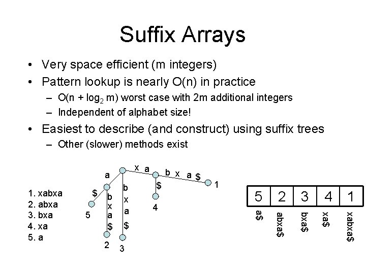
Suffix Arrays • Very space efficient (m integers) • Pattern lookup is nearly O(n) in practice – O(n + log 2 m) worst case with 2 m additional integers – Independent of alphabet size! • Easiest to describe (and construct) using suffix trees – Other (slower) methods exist x a a 3 4 1 xabxa$ 3 2 xa$ 2 $ 4 5 bxa$ 5 b x a $ 1 abxa$ $ $ a$ 1. xabxa 2. abxa 3. bxa 4. xa 5. a b x a$

Suffix array construction • Build suffix tree for T$ • Perform “lexical” depth-first search of suffix tree – output the suffix label of each leaf encountered • Therefore suffix array can be constructed in O(m) time.

Suffix array pattern search • If P is in T, then all the locations of P are consecutive suffixes in Pos. • Do binary search in Pos to find P! – – Compare P with suffix Pos(m/2) If lexicographically less, P is in first half of T If lexicographically more, P is in second half of T Iterate!

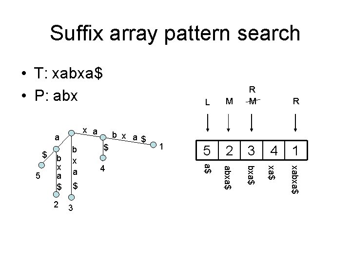
Suffix array pattern search 2 $ 3 4 1 5 2 3 4 1 xabxa$ 5 b x a $ $ xa$ $ b x a$ bxa$ a M abxa$ x a L R M a$ • T: xabxa$ • P: abx R

Suffix array binary search • How long to compare P with suffix of T? – O(n) worst case! • Binary search on Pos takes O(n log m) time • Worst case will be rare – occur if many long prefixes of P appear in T • In random or large alphabet strings – expect to do less than log m comparisons • O(n + log m) running time when combined with LCP table – suffix tree = suffix array + LCP table

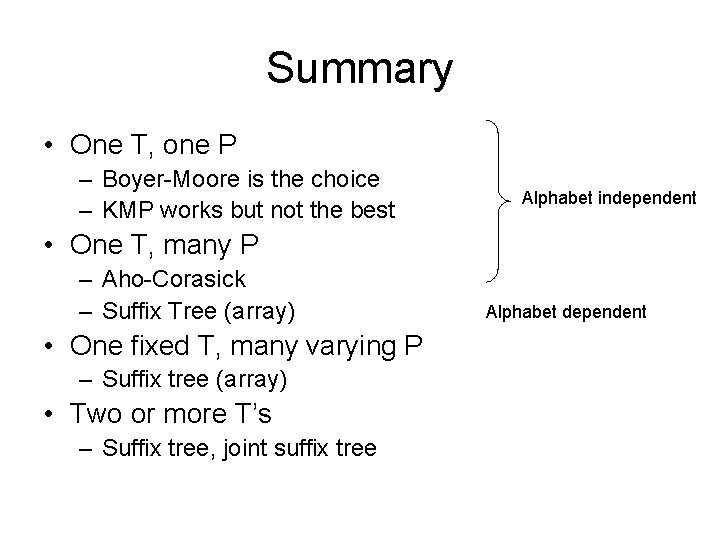
Summary • One T, one P – Boyer-Moore is the choice – KMP works but not the best Alphabet independent • One T, many P – Aho-Corasick – Suffix Tree (array) • One fixed T, many varying P – Suffix tree (array) • Two or more T’s – Suffix tree, joint suffix tree Alphabet dependent