CS 5226 2002 Data Warehouse Performance Tuning Xiaofang


- Slides: 39

CS 5226 2002 Data Warehouse & Performance Tuning Xiaofang Zhou School of Computing, NUS Office: S 16 -08 -20 Email: zhouxf@comp. nus. edu. sg URL: www. itee. uq. edu. au/~zxf

Outline n n Part 1: A review of data warehousing Part 2: Data warehouse tuning 2

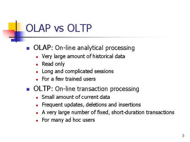
OLAP vs OLTP n OLAP: On-line analytical processing n n n Very large amount of historical data Read only Long and complicated sessions For a few trained users OLTP: On-line transaction processing n n Small amount of current data Frequent updates, deletions and insertions A very large number of fixed, short-duration transactions For many ad hoc users 3

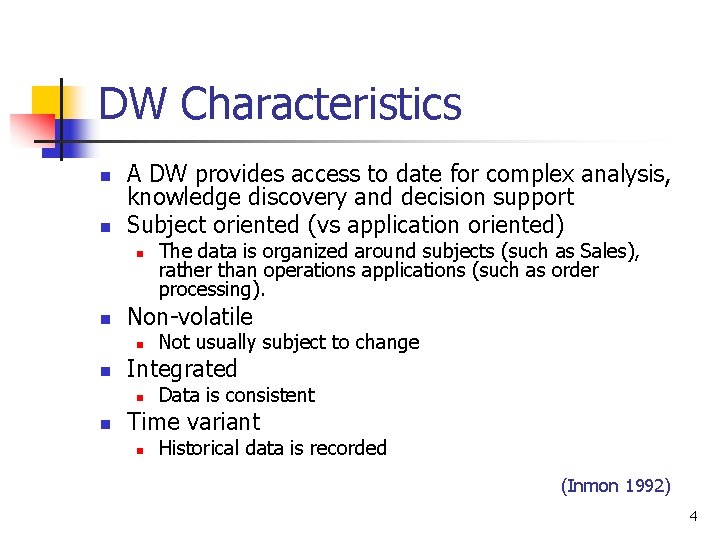
DW Characteristics n n A DW provides access to date for complex analysis, knowledge discovery and decision support Subject oriented (vs application oriented) n n Non-volatile n n Not usually subject to change Integrated n n The data is organized around subjects (such as Sales), rather than operations applications (such as order processing). Data is consistent Time variant n Historical data is recorded (Inmon 1992) 4

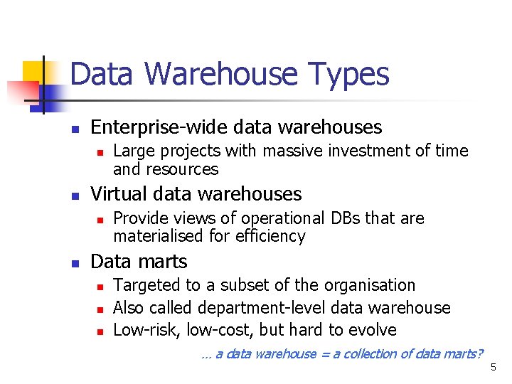
Data Warehouse Types n Enterprise-wide data warehouses n n Virtual data warehouses n n Large projects with massive investment of time and resources Provide views of operational DBs that are materialised for efficiency Data marts n n n Targeted to a subset of the organisation Also called department-level data warehouse Low-risk, low-cost, but hard to evolve … a data warehouse = a collection of data marts? 5

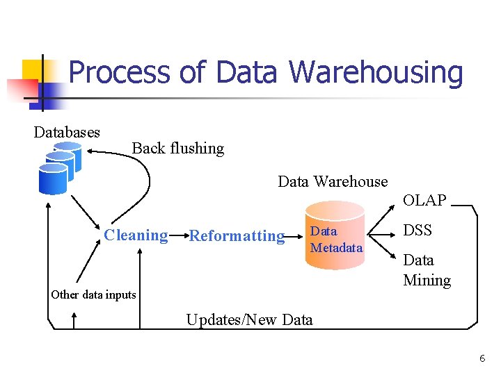
Process of Data Warehousing Databases Back flushing Data Warehouse OLAP Cleaning Reformatting Data Metadata Other data inputs DSS Data Mining Updates/New Data 6

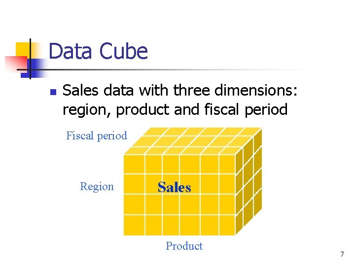
Data Cube n Sales data with three dimensions: region, product and fiscal period Fiscal period Region Sales Product 7

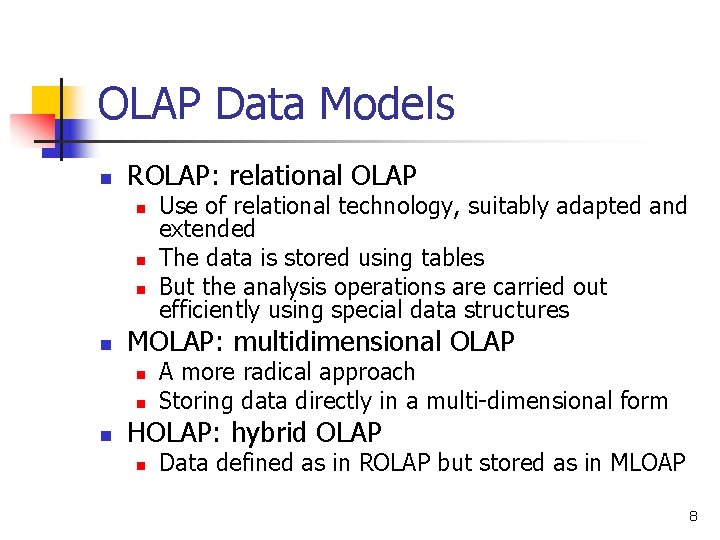
OLAP Data Models n ROLAP: relational OLAP n n MOLAP: multidimensional OLAP n n n Use of relational technology, suitably adapted and extended The data is stored using tables But the analysis operations are carried out efficiently using special data structures A more radical approach Storing data directly in a multi-dimensional form HOLAP: hybrid OLAP n Data defined as in ROLAP but stored as in MLOAP 8

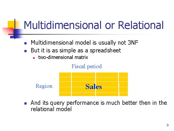
Multidimensional or Relational n n Multidimensional model is usually not 3 NF But it is as simple as a spreadsheet n two-dimensional matrix Fiscal period Region n Sales And its query performance is much better then in the relational model 9

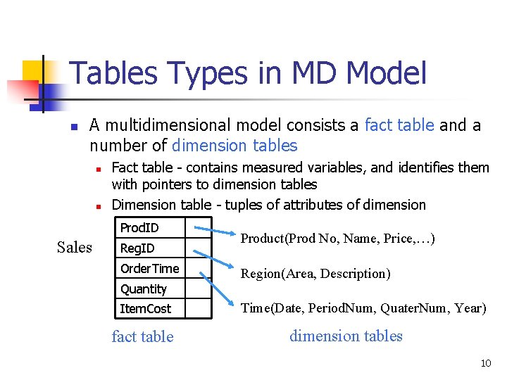
Tables Types in MD Model n A multidimensional model consists a fact table and a number of dimension tables n n Fact table - contains measured variables, and identifies them with pointers to dimension tables Dimension table - tuples of attributes of dimension Prod. ID Sales Reg. ID Order. Time Quantity Item. Cost fact table Product(Prod No, Name, Price, …) Region(Area, Description) Time(Date, Period. Num, Quater. Num, Year) dimension tables 10

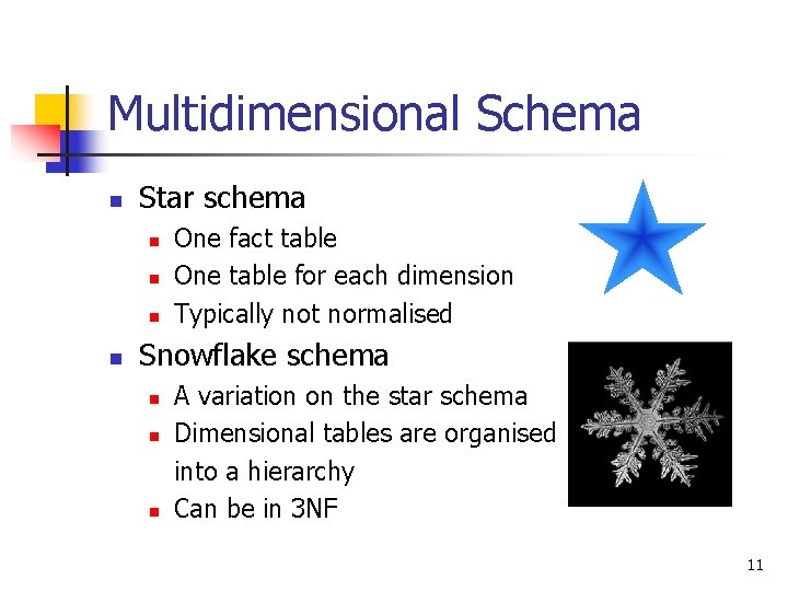
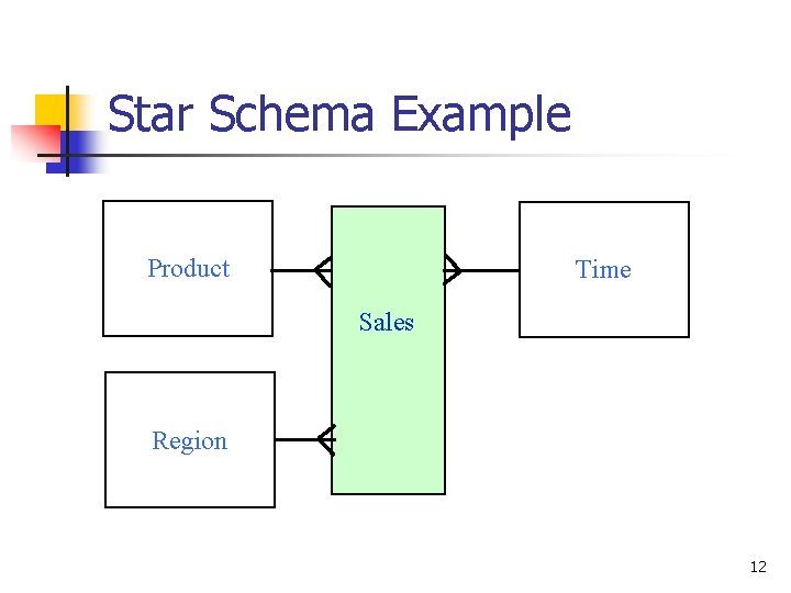
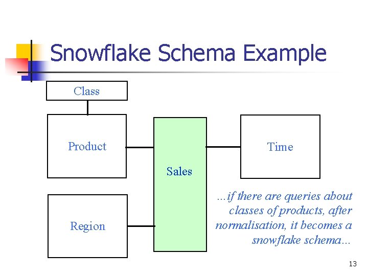
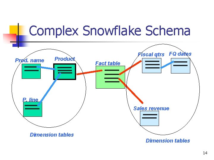
Multidimensional Schema n Star schema n n One fact table One table for each dimension Typically not normalised Snowflake schema n n n A variation on the star schema Dimensional tables are organised into a hierarchy Can be in 3 NF 11

Star Schema Example Product Time Sales Region 12

Snowflake Schema Example Class Product Time Sales Region …if there are queries about classes of products, after normalisation, it becomes a snowflake schema… 13

Complex Snowflake Schema Prod. name Product Fiscal qtrs FQ dates Fact table P. line Sales revenue Dimension tables 14

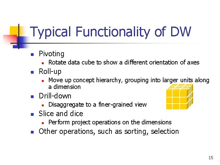
Typical Functionality of DW n Pivoting n n Roll-up n n Disaggregate to a finer-grained view Slice and dice n n Move up concept hierarchy, grouping into larger units along a dimension Drill-down n n Rotate data cube to show a different orientation of axes Perform project operations on the dimensions Other operations, such as sorting, selection 15

Data Warehousing Technology n Aggregate targeting n n n Aggregates flow up from a wide selection of data, and then Targeted decisions flow down Workload type n Broad: aggregate queries over ranges of values n n Deep: queries that require precise individualized information n n E. g. , which frequent flyers have been delayed several times in the last month? Dynamic (vs. Static): queries that require up-to-date information n n E. g. , find the total sales by region and quarter. E. g. . which nodes have the highest traffic now? Main approaches n n n Multidimensional arrays Special indexes – bitmaps and multidimensional indexes Materialised views Optimised foreign key joins Approximation by sampling 16

Tuning Knobs n n n Indexes Materialised views Approximation 17

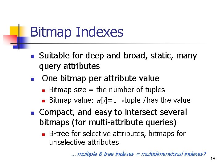
Bitmap Indexes n n Suitable for deep and broad, static, many query attributes One bitmap per attribute value n n n Bitmap size = the number of tuples Bitmap value: a[i]=1 tuple i has the value Compact, and easy to intersect several bitmaps (for multi-attribute queries) n B-tree for selective attributes, bitmaps for unselective attributes … multiple B-tree indexes = multidimensional indexes? 18

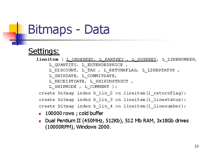
Bitmaps - Data Settings: lineitem ( L_ORDERKEY, L_PARTKEY , L_SUPPKEY, L_LINENUMBER, L_QUANTITY, L_EXTENDEDPRICE , L_DISCOUNT, L_TAX , L_RETURNFLAG, L_LINESTATUS , L_SHIPDATE, L_COMMITDATE, L_RECEIPTDATE, L_SHIPINSTRUCT , L_SHIPMODE , L_COMMENT ); create bitmap index b_lin_2 on lineitem(l_returnflag); create bitmap index b_lin_3 on lineitem(l_linestatus); create bitmap index b_lin_4 on lineitem(l_linenumber); n n 100000 rows ; cold buffer Dual Pentium II (450 MHz, 512 Kb), 512 Mb RAM, 3 x 18 Gb drives (10000 RPM), Windows 2000. 19

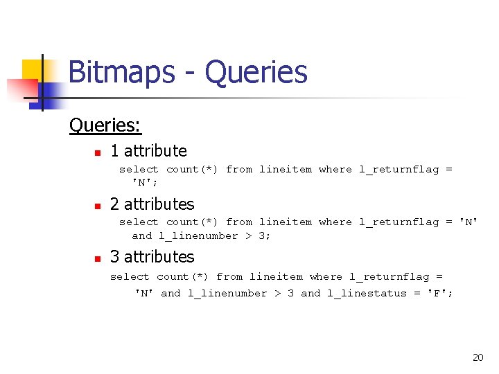
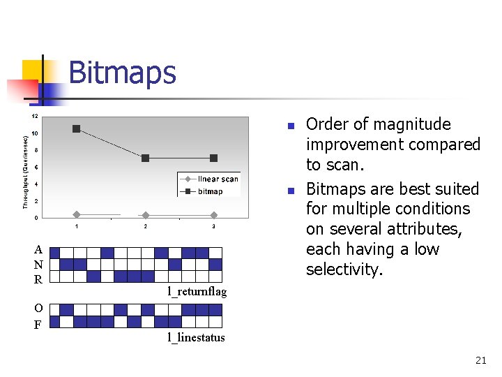
Bitmaps - Queries: n 1 attribute select count(*) from lineitem where l_returnflag = 'N'; n 2 attributes select count(*) from lineitem where l_returnflag = 'N' and l_linenumber > 3; n 3 attributes select count(*) from lineitem where l_returnflag = 'N' and l_linenumber > 3 and l_linestatus = 'F'; 20

Bitmaps n n A N R O F Order of magnitude improvement compared to scan. Bitmaps are best suited for multiple conditions on several attributes, each having a low selectivity. l_returnflag l_linestatus 21

Multidimensional Indexes n n Suitable for deep or broad, static, few query attributes with range queries Examples: quadtrees and R-trees n The space is conceptually organised in grids n n Variable sizes and hierarchical Quadtree: space-centric, regular, recursive decomposition R-tree: data-centric, hierarchical bounding rectangles The problem of “dimensional curse” 22

Multidimensional Indexes Data Settings: create table spatial_facts ( a 1 int, a 2 int, a 3 int, a 4 int, a 5 int, a 6 int, a 7 int, a 8 int, a 9 int, a 10 int, geom_a 3_a 7 mdsys. sdo_geometry ); create index r_spatialfacts on spatial_facts(geom_a 3_a 7) indextype is mdsys. spatial_index; create bitmap index b 2_spatialfacts on spatial_facts(a 3, a 7); n n 500000 rows ; cold buffer Dual Pentium II (450 MHz, 512 Kb), 512 Mb RAM, 3 x 18 Gb drives (10000 RPM), Windows 2000. 23

Multidimensional Indexes Queries: n Point Queries select count(*) from fact where a 3 = 694014 and a 7 = 928878; select count(*) from spatial_facts where SDO_RELATE(geom_a 3_a 7, MDSYS. SDO_GEOMETRY(2001, NULL, MDSYS. SDO_POINT_TYPE(694014, 928878, NULL), 'mask=equal querytype=WINDOW') = 'TRUE'; n Range Queries select count(*) from spatial_facts where SDO_RELATE(geom_a 3_a 7, mdsys. sdo_geometry(2003, NULL, mdsys. sdo_elem_info_array(1, 1003, 3), mdsys. sdo_ordinate_array (10, 800000, 1000000)), 'mask=inside querytype=WINDOW') = 'TRUE'; select count(*) from spatial_facts where a 3 > 10 and a 3 < 1000000 and a 7 > 800000 and a 7 < 1000000; 24

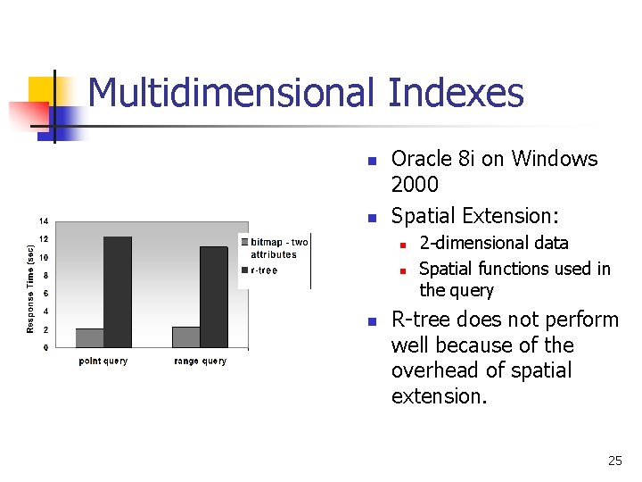
Multidimensional Indexes n n Oracle 8 i on Windows 2000 Spatial Extension: n n n 2 -dimensional data Spatial functions used in the query R-tree does not perform well because of the overhead of spatial extension. 25

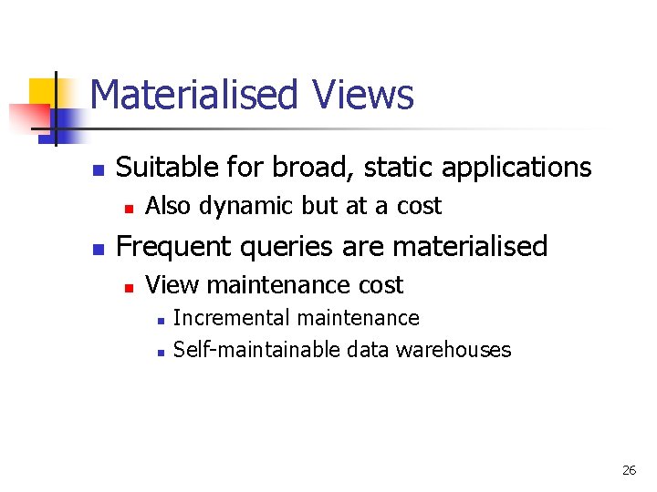
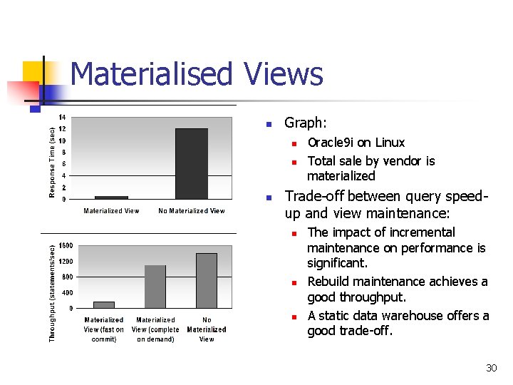
Materialised Views n Suitable for broad, static applications n n Also dynamic but at a cost Frequent queries are materialised n View maintenance cost n n Incremental maintenance Self-maintainable data warehouses 26

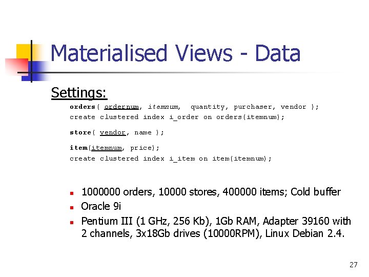
Materialised Views - Data Settings: orders( ordernum, itemnum, quantity, purchaser, vendor ); create clustered index i_order on orders(itemnum); store( vendor, name ); item(itemnum, price); create clustered index i_item on item(itemnum); n n n 1000000 orders, 10000 stores, 400000 items; Cold buffer Oracle 9 i Pentium III (1 GHz, 256 Kb), 1 Gb RAM, Adapter 39160 with 2 channels, 3 x 18 Gb drives (10000 RPM), Linux Debian 2. 4. 27

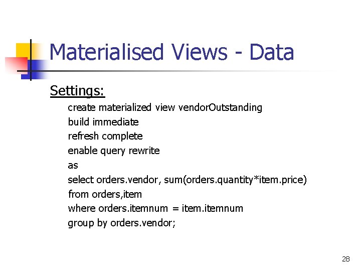
Materialised Views - Data Settings: create materialized view vendor. Outstanding build immediate refresh complete enable query rewrite as select orders. vendor, sum(orders. quantity*item. price) from orders, item where orders. itemnum = itemnum group by orders. vendor; 28

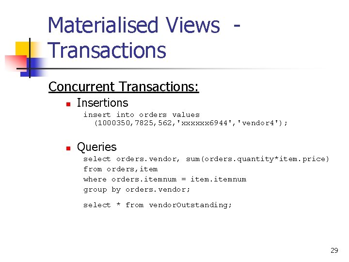
Materialised Views Transactions Concurrent Transactions: n Insertions insert into orders values (1000350, 7825, 562, 'xxxxxx 6944', 'vendor 4'); n Queries select orders. vendor, sum(orders. quantity*item. price) from orders, item where orders. itemnum = itemnum group by orders. vendor; select * from vendor. Outstanding; 29

Materialised Views n Graph: n n n Oracle 9 i on Linux Total sale by vendor is materialized Trade-off between query speedup and view maintenance: n n n The impact of incremental maintenance on performance is significant. Rebuild maintenance achieves a good throughput. A static data warehouse offers a good trade-off. 30

Materialised View Maintenance n n Problem when large number of views to maintain. The order in which views are maintained is important: n A view can be computed from an existing view instead of being recomputed from the base relations (total per region can be computed from total per nation). n n Let the views and base tables be nodes v_i Let there be an edge from v_1 to v_2 if it possible to compute the view v_2 from v_1. Associate the cost of computing v_2 from v_1 to this edge. Compute all pairs shortest path where the start nodes are the set of base tables. The result is an acyclic graph A. Take a topological sort of A and let that be the order of view construction. 31

Result Approximation n n Suitable for broad, dynamic, large data Examples n n n When computing the average, one can increase sample sizes until no significant change of the value Increased accuracy with time Approximated results within given error bounds 32

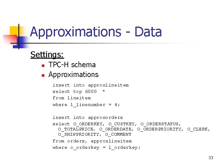
Approximations - Data Settings: n n TPC-H schema Approximations insert into approxlineitem select top 6000 * from lineitem where l_linenumber = 4; insert into approxorders select O_ORDERKEY, O_CUSTKEY, O_ORDERSTATUS, O_TOTALPRICE, O_ORDERDATE, O_ORDERPRIORITY, O_CLERK, O_SHIPPRIORITY, O_COMMENT from orders, approxlineitem where o_orderkey = l_orderkey; 33

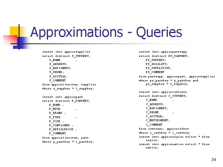
Approximations - Queries insert into approxsupplier select distinct S_SUPPKEY, S_NAME , S_ADDRESS, S_NATIONKEY, S_PHONE, S_ACCTBAL, S_COMMENT from approxlineitem, supplier where s_suppkey = l_suppkey; insert into approxpart select distinct P_PARTKEY, P_NAME , P_MFGR , P_BRAND , P_TYPE , P_SIZE , P_CONTAINER , P_RETAILPRICE , P_COMMENT from approxlineitem, part where p_partkey = l_partkey; insert into approxpartsupp select distinct PS_PARTKEY, PS_SUPPKEY, PS_AVAILQTY, PS_SUPPLYCOST, PS_COMMENT from partsupp, approxpart, approxsupplier where ps_partkey = p_partkey and ps_suppkey = s_suppkey; insert into approxcustomer select distinct C_CUSTKEY, C_NAME , C_ADDRESS, C_NATIONKEY, C_PHONE , C_ACCTBAL, C_MKTSEGMENT, C_COMMENT from customer, approxorders where o_custkey = c_custkey; insert into approxregion select * from region; insert into approxnation select * from nation; 34

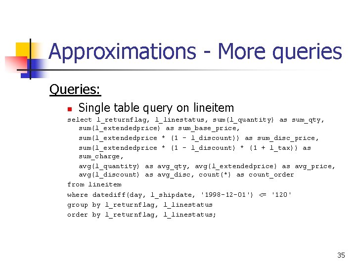
Approximations - More queries Queries: n Single table query on lineitem select l_returnflag, l_linestatus, sum(l_quantity) as sum_qty, sum(l_extendedprice) as sum_base_price, sum(l_extendedprice * (1 - l_discount)) as sum_disc_price, sum(l_extendedprice * (1 - l_discount) * (1 + l_tax)) as sum_charge, avg(l_quantity) as avg_qty, avg(l_extendedprice) as avg_price, avg(l_discount) as avg_disc, count(*) as count_order from lineitem where datediff(day, l_shipdate, '1998 -12 -01') <= '120' group by l_returnflag, l_linestatus order by l_returnflag, l_linestatus; 35

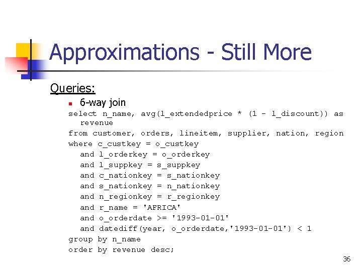
Approximations - Still More Queries: n 6 -way join select n_name, avg(l_extendedprice * (1 - l_discount)) as revenue from customer, orders, lineitem, supplier, nation, region where c_custkey = o_custkey and l_orderkey = o_orderkey and l_suppkey = s_suppkey and c_nationkey = s_nationkey and s_nationkey = n_nationkey and n_regionkey = r_regionkey and r_name = 'AFRICA' and o_orderdate >= '1993 -01 -01' and datediff(year, o_orderdate, '1993 -01 -01') < 1 group by n_name order by revenue desc; 36

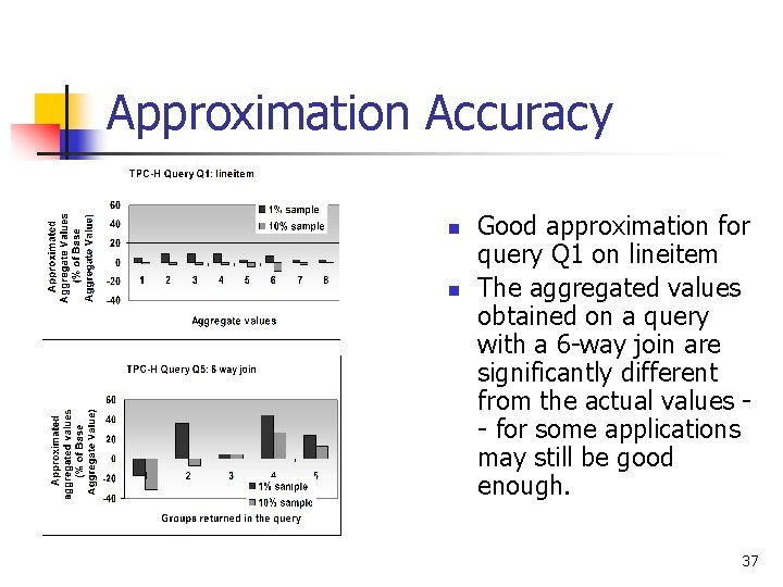
Approximation Accuracy n n Good approximation for query Q 1 on lineitem The aggregated values obtained on a query with a 6 -way join are significantly different from the actual values - for some applications may still be good enough. 37

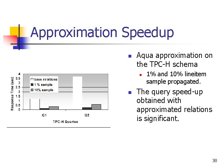
Approximation Speedup n Aqua approximation on the TPC-H schema n n 1% and 10% lineitem sample propagated. The query speed-up obtained with approximated relations is significant. 38

Summary n In this module, we have covered: n n n Basic concepts of data warehousing Data warehousing technologies How to optimise data warehouse performance 39