CS 478 Tools for Machine Learning and Data

CS 478 – Tools for Machine Learning and Data Mining Linear and Logistic Regression (Adapted from various sources) (e. g. , Luiz Pessoa PY 206 class at Brown University)

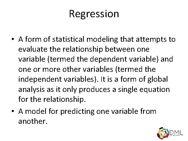
Regression • A form of statistical modeling that attempts to evaluate the relationship between one variable (termed the dependent variable) and one or more other variables (termed the independent variables). It is a form of global analysis as it only produces a single equation for the relationship. • A model for predicting one variable from another.

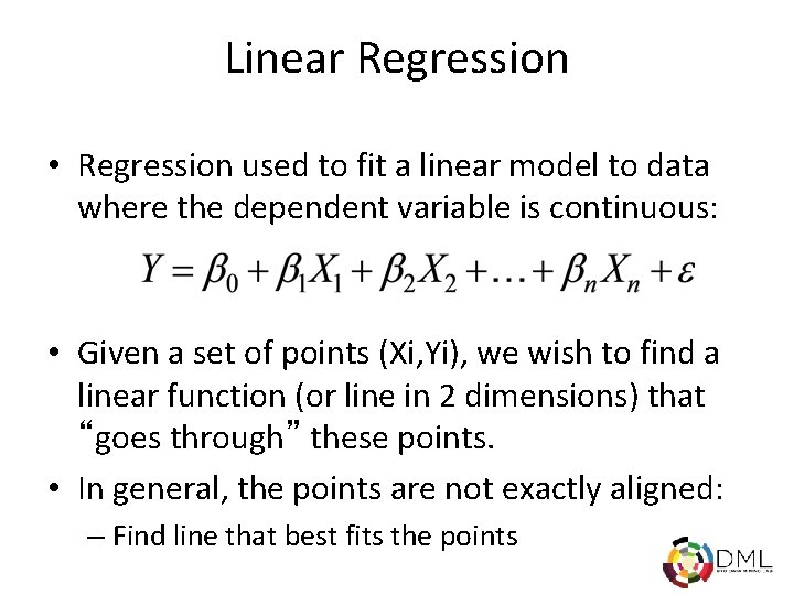
Linear Regression • Regression used to fit a linear model to data where the dependent variable is continuous: • Given a set of points (Xi, Yi), we wish to find a linear function (or line in 2 dimensions) that “goes through” these points. • In general, the points are not exactly aligned: – Find line that best fits the points

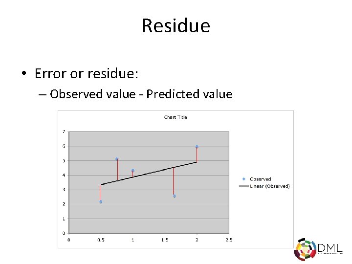
Residue • Error or residue: – Observed value - Predicted value

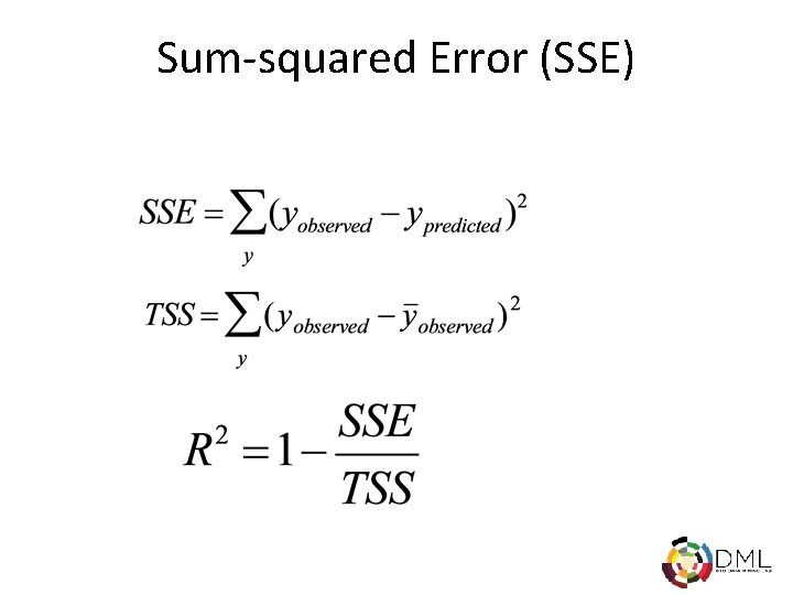
Sum-squared Error (SSE)

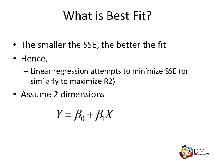
What is Best Fit? • The smaller the SSE, the better the fit • Hence, – Linear regression attempts to minimize SSE (or similarly to maximize R 2) • Assume 2 dimensions

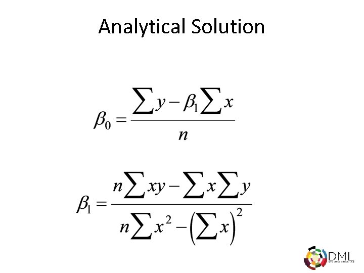
Analytical Solution

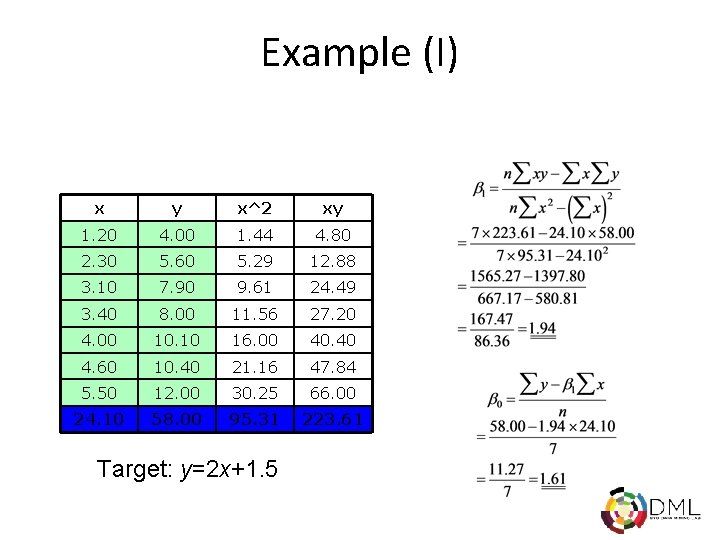
Example (I) x y x^2 xy 1. 20 4. 00 1. 44 4. 80 2. 30 5. 60 5. 29 12. 88 3. 10 7. 90 9. 61 24. 49 3. 40 8. 00 11. 56 27. 20 4. 00 10. 10 16. 00 40. 40 4. 60 10. 40 21. 16 47. 84 5. 50 12. 00 30. 25 66. 00 24. 10 58. 00 95. 31 223. 61 Target: y=2 x+1. 5

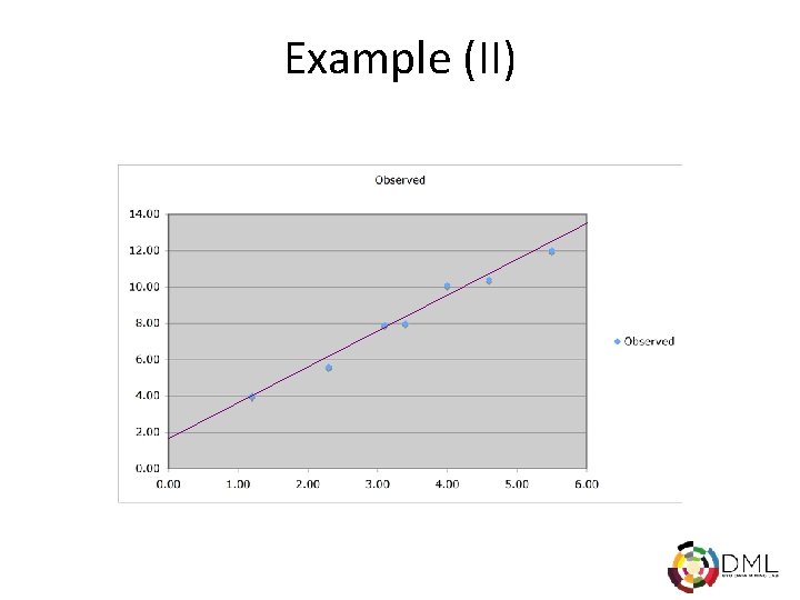
Example (II)

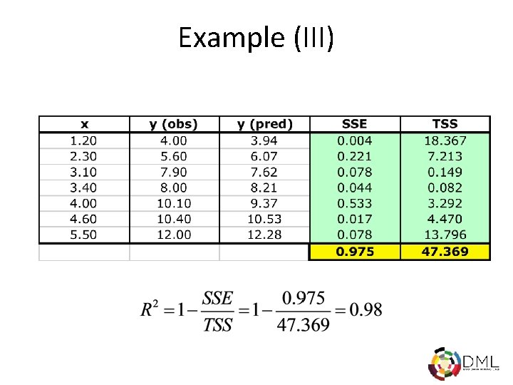
Example (III)

Logistic Regression • Regression used to fit a curve to data in which the dependent variable is binary, or dichotomous • Typical application: Medicine – We might want to predict response to treatment, where we might code survivors as 1 and those who don’t survive as 0

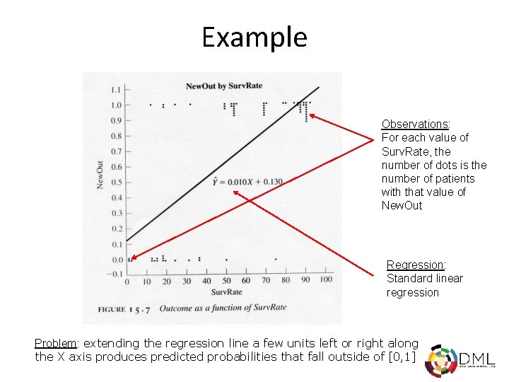
Example Observations: For each value of Surv. Rate, the number of dots is the number of patients with that value of New. Out Regression: Standard linear regression Problem: extending the regression line a few units left or right along the X axis produces predicted probabilities that fall outside of [0, 1]

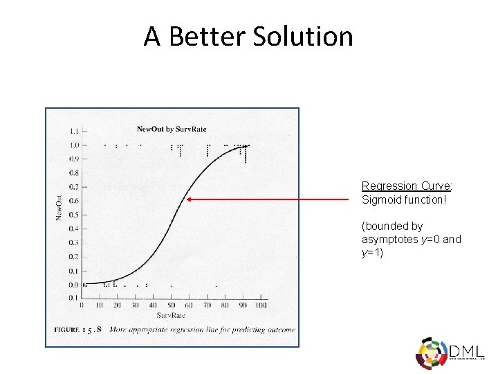
A Better Solution Regression Curve: Sigmoid function! (bounded by asymptotes y=0 and y=1)

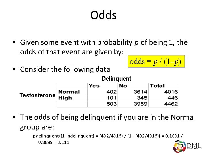
Odds • Given some event with probability p of being 1, the odds of that event are given by: odds = p / (1–p) • Consider the following data Delinquent Testosterone • The odds of being delinquent if you are in the Normal group are: pdelinquent/(1–pdelinquent) = (402/4016) / (1 - (402/4016)) = 0. 1001 / 0. 8889 = 0. 111

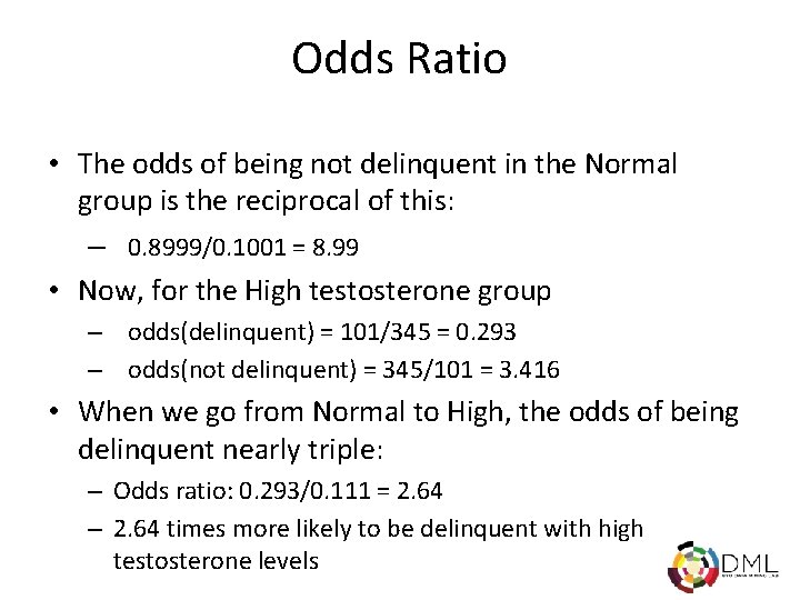
Odds Ratio • The odds of being not delinquent in the Normal group is the reciprocal of this: – 0. 8999/0. 1001 = 8. 99 • Now, for the High testosterone group – odds(delinquent) = 101/345 = 0. 293 – odds(not delinquent) = 345/101 = 3. 416 • When we go from Normal to High, the odds of being delinquent nearly triple: – Odds ratio: 0. 293/0. 111 = 2. 64 – 2. 64 times more likely to be delinquent with high testosterone levels

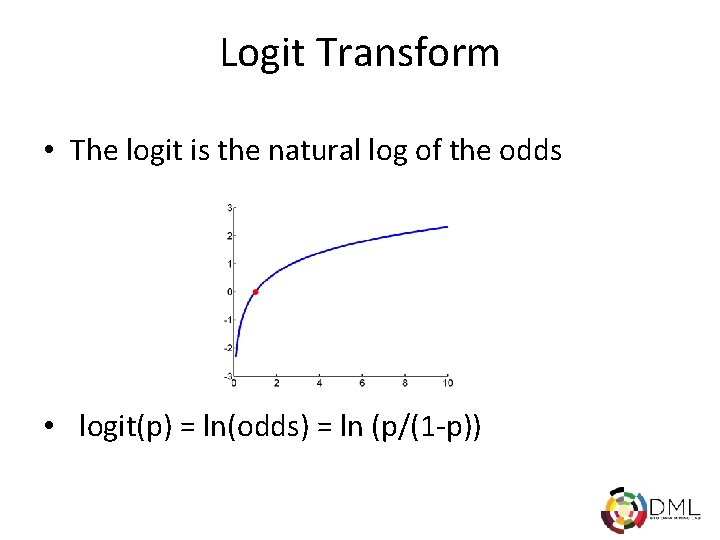
Logit Transform • The logit is the natural log of the odds • logit(p) = ln(odds) = ln (p/(1 -p))

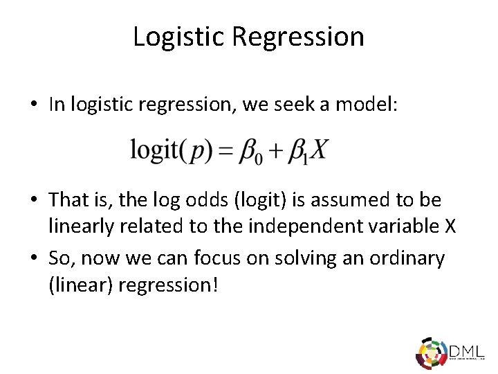
Logistic Regression • In logistic regression, we seek a model: • That is, the log odds (logit) is assumed to be linearly related to the independent variable X • So, now we can focus on solving an ordinary (linear) regression!

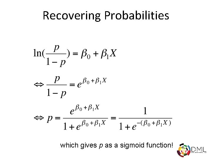
Recovering Probabilities which gives p as a sigmoid function!

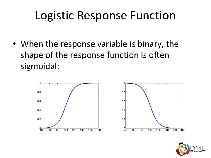
Logistic Response Function • When the response variable is binary, the shape of the response function is often sigmoidal:

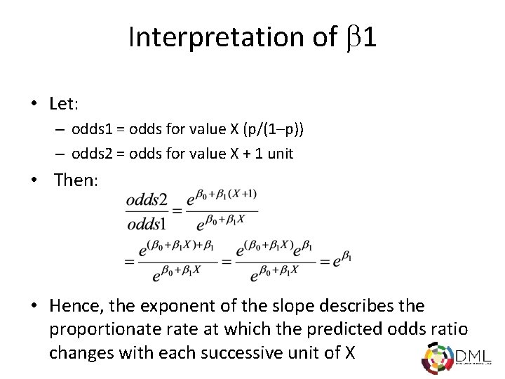
Interpretation of 1 • Let: – odds 1 = odds for value X (p/(1–p)) – odds 2 = odds for value X + 1 unit • Then: • Hence, the exponent of the slope describes the proportionate rate at which the predicted odds ratio changes with each successive unit of X

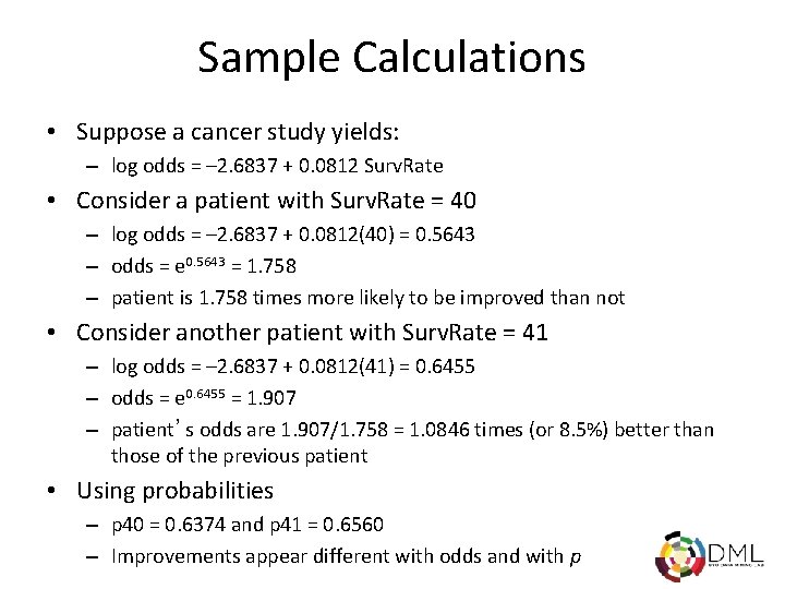
Sample Calculations • Suppose a cancer study yields: – log odds = – 2. 6837 + 0. 0812 Surv. Rate • Consider a patient with Surv. Rate = 40 – log odds = – 2. 6837 + 0. 0812(40) = 0. 5643 – odds = e 0. 5643 = 1. 758 – patient is 1. 758 times more likely to be improved than not • Consider another patient with Surv. Rate = 41 – log odds = – 2. 6837 + 0. 0812(41) = 0. 6455 – odds = e 0. 6455 = 1. 907 – patient’s odds are 1. 907/1. 758 = 1. 0846 times (or 8. 5%) better than those of the previous patient • Using probabilities – p 40 = 0. 6374 and p 41 = 0. 6560 – Improvements appear different with odds and with p

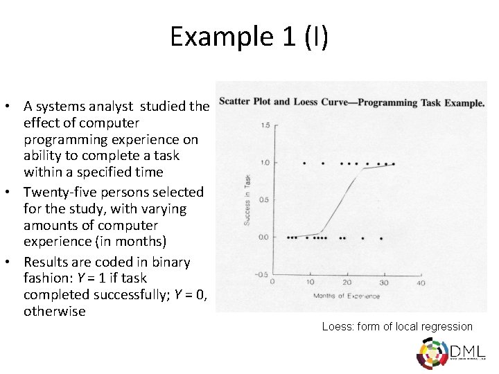
Example 1 (I) • A systems analyst studied the effect of computer programming experience on ability to complete a task within a specified time • Twenty-five persons selected for the study, with varying amounts of computer experience (in months) • Results are coded in binary fashion: Y = 1 if task completed successfully; Y = 0, otherwise Loess: form of local regression

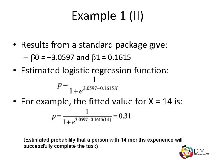
Example 1 (II) • Results from a standard package give: – 0 = – 3. 0597 and 1 = 0. 1615 • Estimated logistic regression function: • For example, the fitted value for X = 14 is: (Estimated probability that a person with 14 months experience will successfully complete the task)

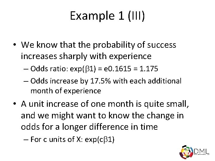
Example 1 (III) • We know that the probability of success increases sharply with experience – Odds ratio: exp( 1) = e 0. 1615 = 1. 175 – Odds increase by 17. 5% with each additional month of experience • A unit increase of one month is quite small, and we might want to know the change in odds for a longer difference in time – For c units of X: exp(c 1)

Example 1 (IV) • Suppose we want to compare individuals with relatively little experience to those with extensive experience, say 10 months versus 25 months (c = 15) – Odds ratio: e 15 x 0. 1615 = 11. 3 – Odds of completing the task increase 11 -fold!

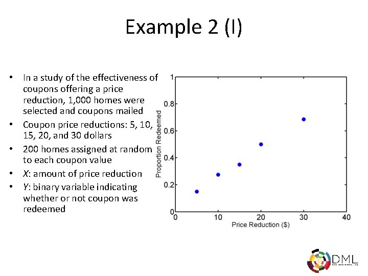
Example 2 (I) • In a study of the effectiveness of coupons offering a price reduction, 1, 000 homes were selected and coupons mailed • Coupon price reductions: 5, 10, 15, 20, and 30 dollars • 200 homes assigned at random to each coupon value • X: amount of price reduction • Y: binary variable indicating whether or not coupon was redeemed

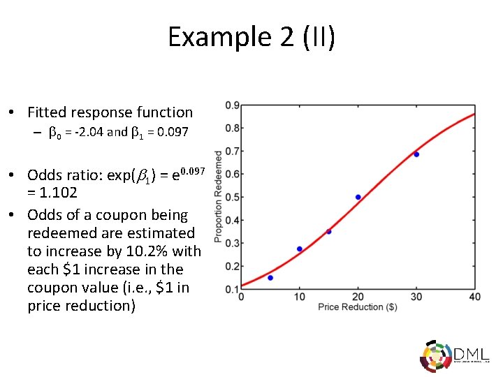
Example 2 (II) • Fitted response function – 0 = -2. 04 and 1 = 0. 097 • Odds ratio: exp( 1) = e 0. 097 = 1. 102 • Odds of a coupon being redeemed are estimated to increase by 10. 2% with each $1 increase in the coupon value (i. e. , $1 in price reduction)

Putting it to Work • For each value of X, you may not have probability but rather a number of <x, y> pairs from which you can extract frequencies and hence probabilities – Raw data: <12, 0>, <12, 1>, <14, 1>, <12, 0> – Probability data (p=1, 3 rd entry is number of occurrences in raw data): <12, 0. 4, 5>, <14, 0. 66, 3> – Odds ratio data…

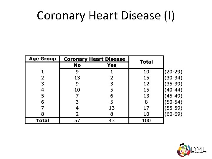
Coronary Heart Disease (I)

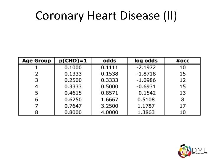
Coronary Heart Disease (II)

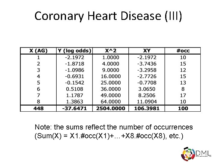
Coronary Heart Disease (III) Note: the sums reflect the number of occurrences (Sum(X) = X 1. #occ(X 1)+…+X 8. #occ(X 8), etc. )

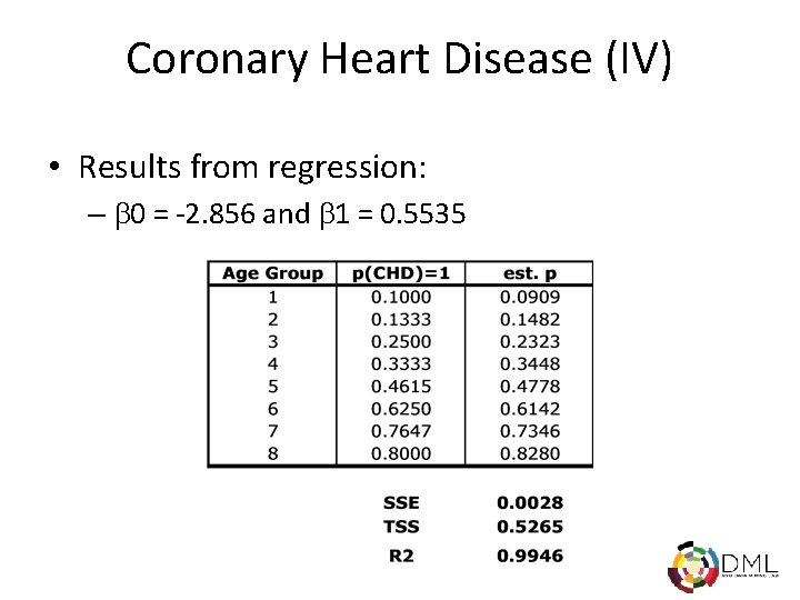
Coronary Heart Disease (IV) • Results from regression: – 0 = -2. 856 and 1 = 0. 5535

Summary • Regression is a powerful data mining technique – It provides prediction – It offers insight on the relative power of each variable • We have focused on the case of a single independent variable – What about the general case?