CS 473 Algorithms I Lecture X Ackermanns Function

CS 473 -Algorithms I Lecture X Ackermann’s Function and Its Inverse CS 473 Lecture X 1

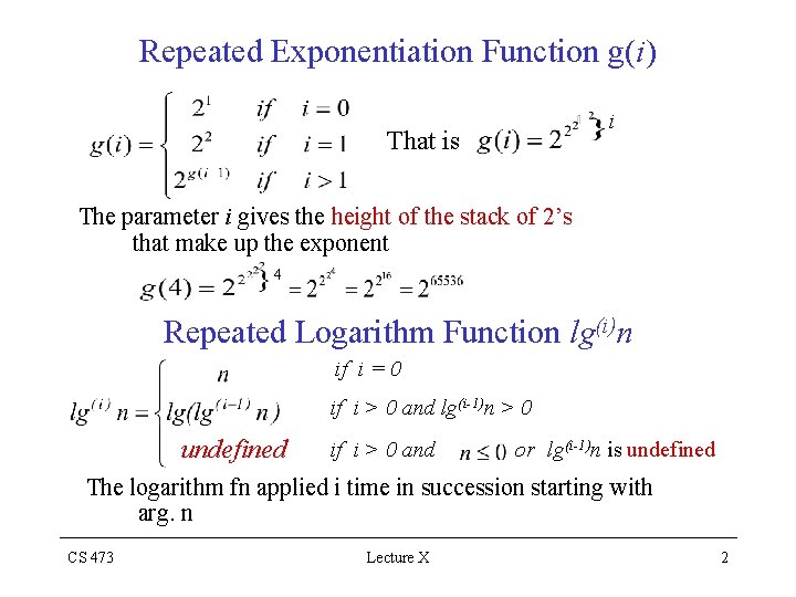
Repeated Exponentiation Function g(i) i That is The parameter i gives the height of the stack of 2’s that make up the exponent 4 Repeated Logarithm Function lg(i)n if i = 0 if i > 0 and lg(i-1)n > 0 undefined if i > 0 and or lg(i-1)n is undefined The logarithm fn applied i time in succession starting with arg. n CS 473 Lecture X 2

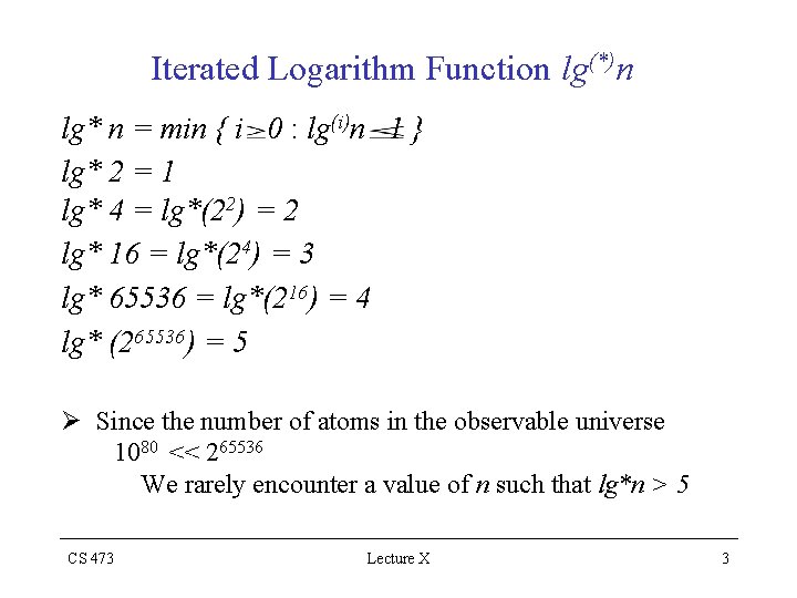
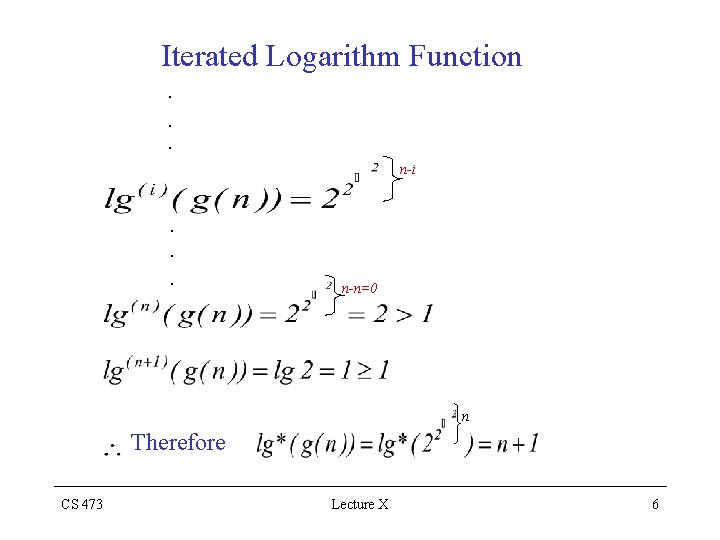
Iterated Logarithm Function lg(*)n lg* n = min { i 0 : lg(i)n 1 } lg* 2 = 1 lg* 4 = lg*(22) = 2 lg* 16 = lg*(24) = 3 lg* 65536 = lg*(216) = 4 lg* (265536) = 5 Ø Since the number of atoms in the observable universe 1080 << 265536 We rarely encounter a value of n such that lg*n > 5 CS 473 Lecture X 3

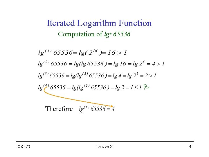
Iterated Logarithm Function Computation of lg* 65536 P Therefore CS 473 Lecture X 4

Iterated Logarithm Function The lg*n fn is essentially the inverse of repeated exponentiation n where n n n-1 n-2 CS 473 Lecture X n-2 n-3 5

Iterated Logarithm Function. . . n-i . . . n-n=0 n Therefore CS 473 Lecture X 6

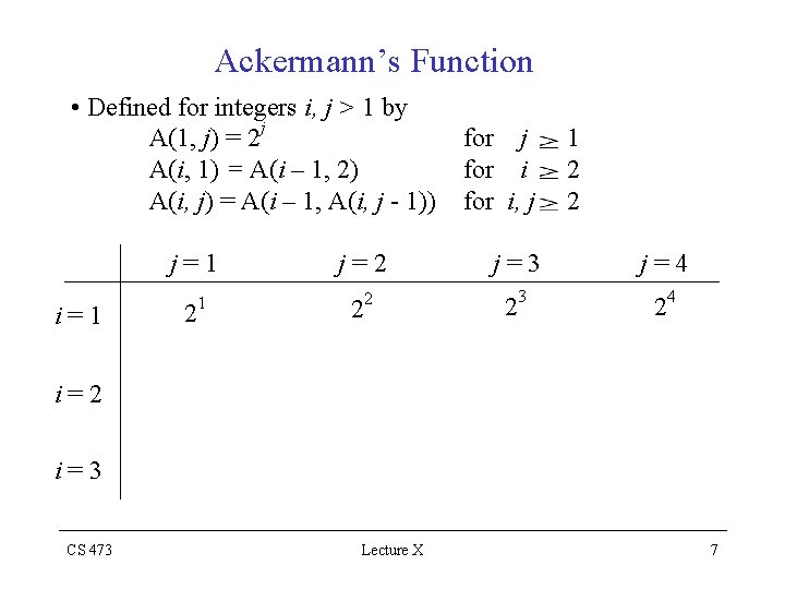
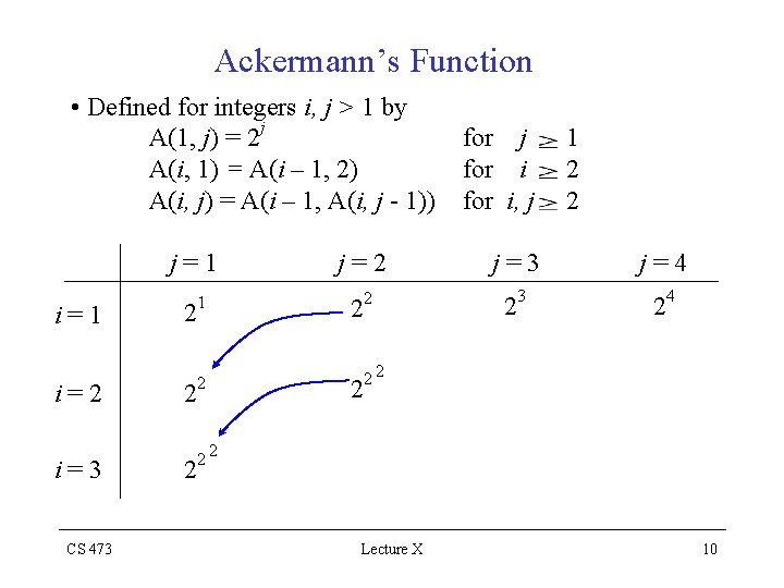
Ackermann’s Function • Defined for integers i, j > 1 by A(1, j) = 2 j A(i, 1) = A(i – 1, 2) A(i, j) = A(i – 1, A(i, j - 1)) j=1 i=1 1 2 for j for i, j 1 2 2 j=3 j=4 22 23 24 i=2 i=3 CS 473 Lecture X 7

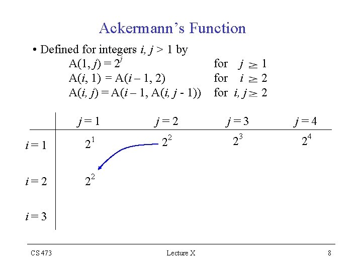
Ackermann’s Function • Defined for integers i, j > 1 by A(1, j) = 2 j A(i, 1) = A(i – 1, 2) A(i, j) = A(i – 1, A(i, j - 1)) j=1 1 i=1 2 i=2 22 for j for i, j 1 2 2 j=3 j=4 22 23 24 i=3 CS 473 Lecture X 8

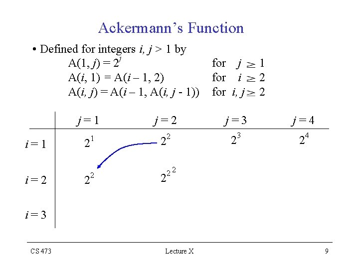
Ackermann’s Function • Defined for integers i, j > 1 by A(1, j) = 2 j A(i, 1) = A(i – 1, 2) A(i, j) = A(i – 1, A(i, j - 1)) j=1 i=2 1 2 2 2 for j for i, j 1 2 2 j=3 j=4 22 23 24 22 2 i=3 CS 473 Lecture X 9

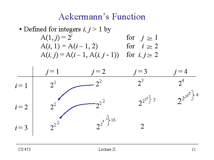
Ackermann’s Function • Defined for integers i, j > 1 by A(1, j) = 2 j A(i, 1) = A(i – 1, 2) A(i, j) = A(i – 1, A(i, j - 1)) j=1 i=2 i=3 CS 473 1 2 2 2 for j for i, j 1 2 2 j=3 j=4 22 23 24 22 2 Lecture X 10

Ackermann’s Function • Defined for integers i, j > 1 by A(1, j) = 2 j A(i, 1) = A(i – 1, 2) A(i, j) = A(i – 1, A(i, j - 1)) j=1 i=2 i=3 CS 473 1 2 22 22 for j for i, j 1 2 2 j=3 j=4 22 23 24 4 3 22 2 16 2 Lecture X 2 11

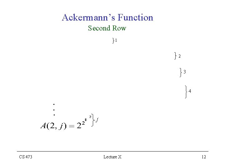
Ackermann’s Function Second Row 1 2 3 4 . . . CS 473 j Lecture X 12

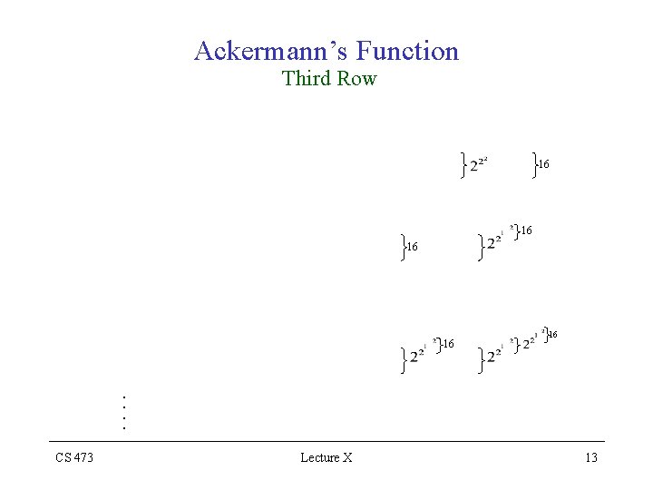
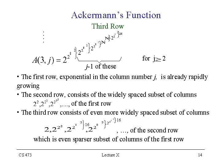
Ackermann’s Function Third Row 16 16 16 ∙ ∙ CS 473 Lecture X 13

Ackermann’s Function Third Row ∙ ∙ 16 for j 2 j-1 of these • The first row, exponential in the column number j, is already rapidly growing • The second row, consists of the widely spaced subset of columns of the first row • The third row consists of even more widely spaced subset of columns 16 16 , …, of the second row which is even sparser subset of columns of the first row CS 473 Lecture X 14

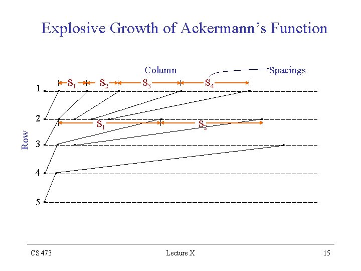
Explosive Growth of Ackermann’s Function 1 Row 2 S 1 S 2 Column S 3 S 1 Spacings S 4 S 2 3 4 5 CS 473 Lecture X 15

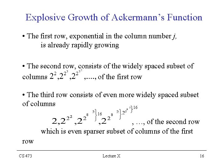
Explosive Growth of Ackermann’s Function • The first row, exponential in the column number j, is already rapidly growing • The second row, consists of the widely spaced subset of columns of the first row • The third row consists of even more widely spaced subset of columns 16 16 , …, of the second row which is even sparser subset of columns of the first row CS 473 Lecture X 16

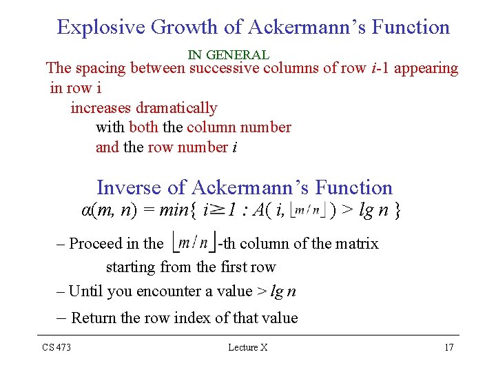
Explosive Growth of Ackermann’s Function IN GENERAL The spacing between successive columns of row i-1 appearing in row i increases dramatically with both the column number and the row number i Inverse of Ackermann’s Function α(m, n) = min{ i 1 : A( i, ) > lg n } – Proceed in the -th column of the matrix starting from the first row – Until you encounter a value > lg n – Return the row index of that value CS 473 Lecture X 17

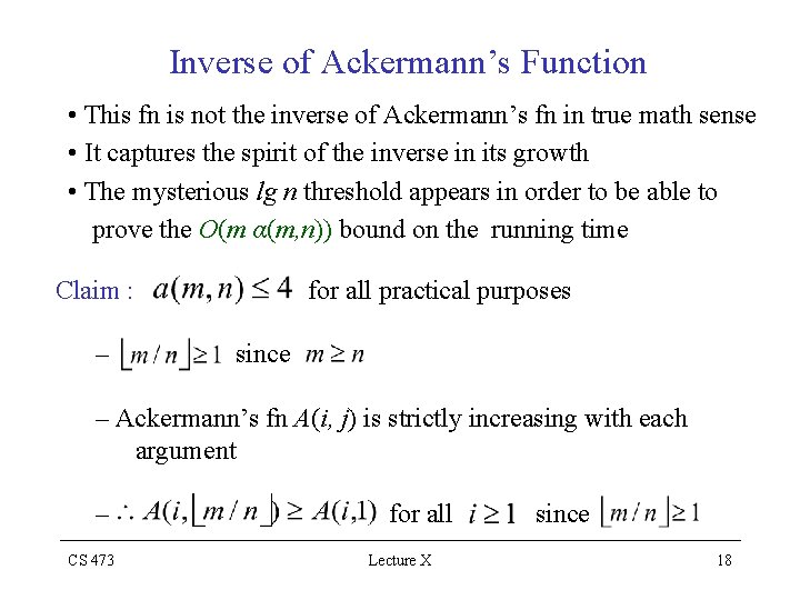
Inverse of Ackermann’s Function • This fn is not the inverse of Ackermann’s fn in true math sense • It captures the spirit of the inverse in its growth • The mysterious lg n threshold appears in order to be able to prove the O(m α(m, n)) bound on the running time Claim : – for all practical purposes since – Ackermann’s fn A(i, j) is strictly increasing with each argument – CS 473 for all Lecture X since 18

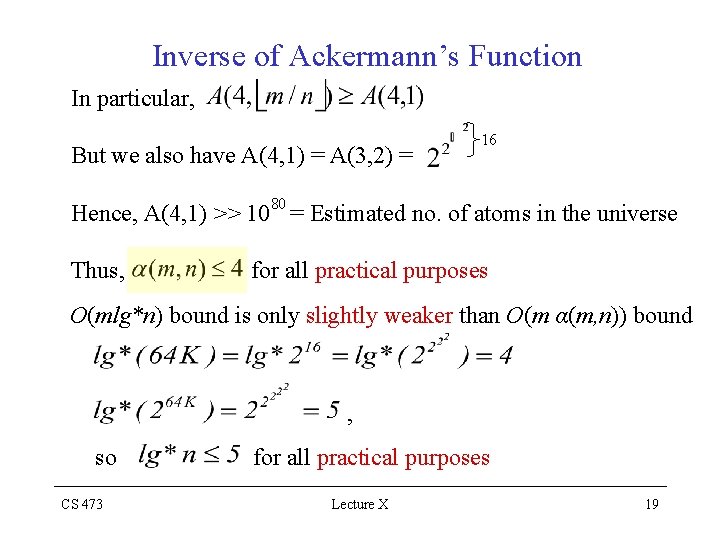
Inverse of Ackermann’s Function In particular, But we also have A(4, 1) = A(3, 2) = 16 Hence, A(4, 1) >> 1080 = Estimated no. of atoms in the universe Thus, for all practical purposes O(mlg*n) bound is only slightly weaker than O(m α(m, n)) bound , so CS 473 for all practical purposes Lecture X 19

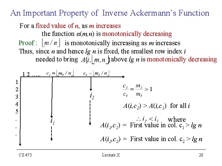
An Important Property of Inverse Ackermann’s Function For a fixed value of n, as m increases the function α(m, n) is monotonically decreasing Proof : is monotonically increasing as m increases Thus, since n and hence lg n is fixed, the smallest row index i needed to bring above lg n is monotonically decreasing 1 2 …. . 1 2 3 4 5. . . 1 i 2 A(i, c 2) > A(i, c 1) for all i i 1 where A(i 1, c 1) = First value in col. c 1 > lg n A(i 2, c 2) = First value in col. c 2 > lg n CS 473 Lecture X 20

An Important Property of Inverse Ackermann’s Function • This property corresponds to our intuition about disjoint set forests with path compression • We would expect the average FIND-PATH length to decrease due to path compression • If we perform m operations in time O(m α(m, n)) then, the average time per operation is O(α(m, n)) which is monotonically decreasing as m increases CS 473 Lecture X 21