CS 4501 Introduction to Computer Vision Epipolar Geometry



- Slides: 52

CS 4501: Introduction to Computer Vision Epipolar Geometry: Essential Matrix Various slides from previous courses by: D. A. Forsyth (Berkeley / UIUC), I. Kokkinos (Ecole Centrale / UCL). S. Lazebnik (UNC / UIUC), S. Seitz (MSR / Facebook), J. Hays (Brown / Georgia Tech), A. Berg (Stony Brook / UNC), D. Samaras (Stony Brook). J. M. Frahm (UNC), V. Ordonez (UVA), Steve Seitz (UW).

Last Class • Stereo Vision – Dense Stereo • More on Epipolar Geometry

Today’s Class • More on Epipolar Geometry • Essential Matrix • Fundamental Matrix

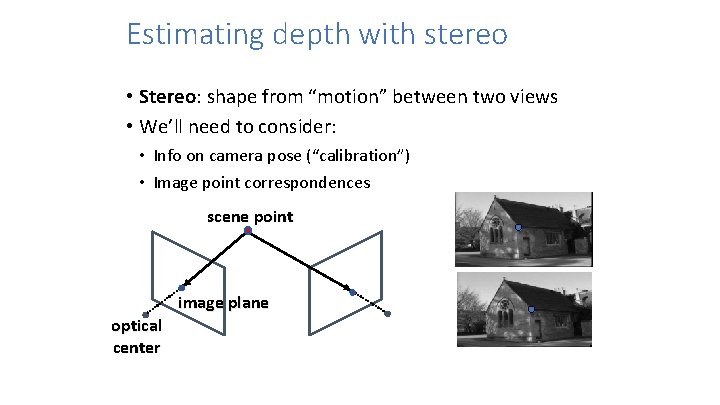
Estimating depth with stereo • Stereo: shape from “motion” between two views • We’ll need to consider: • Info on camera pose (“calibration”) • Image point correspondences scene point image plane optical center

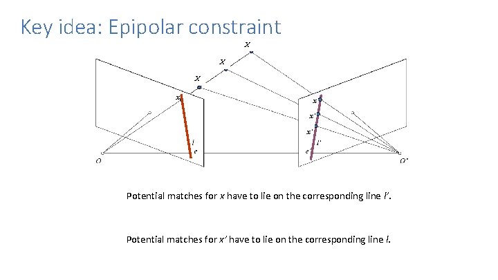
Key idea: Epipolar constraint X X X x x’ x’ x’ Potential matches for x have to lie on the corresponding line l’. Potential matches for x’ have to lie on the corresponding line l.

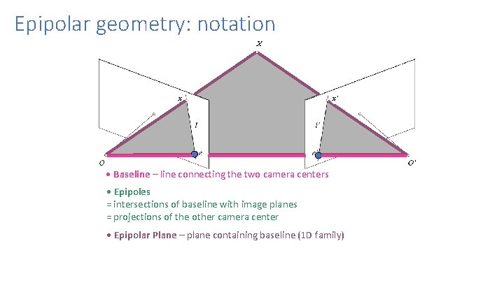
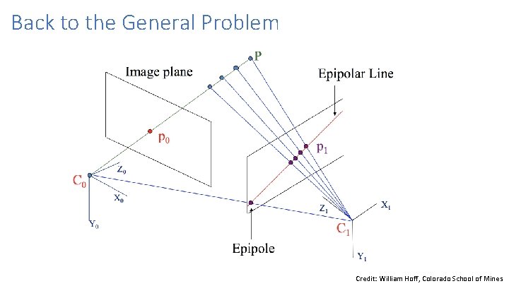
Epipolar geometry: notation X x x’ • Baseline – line connecting the two camera centers • Epipoles = intersections of baseline with image planes = projections of the other camera center • Epipolar Plane – plane containing baseline (1 D family)

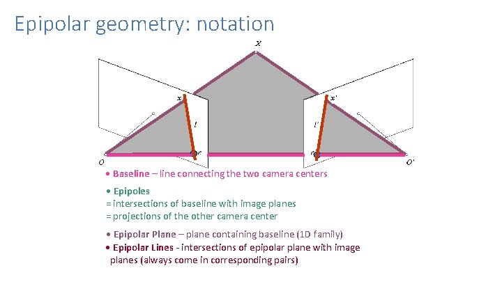
Epipolar geometry: notation X x x’ • Baseline – line connecting the two camera centers • Epipoles = intersections of baseline with image planes = projections of the other camera center • Epipolar Plane – plane containing baseline (1 D family) • Epipolar Lines - intersections of epipolar plane with image planes (always come in corresponding pairs)

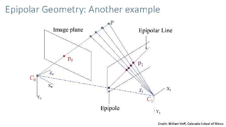
Epipolar Geometry: Another example Credit: William Hoff, Colorado School of Mines

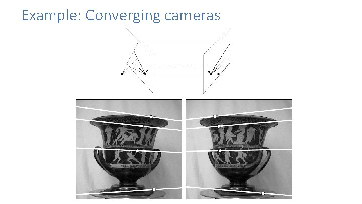
Example: Converging cameras

Geometry for a simple stereo system • First, assuming parallel optical axes, known camera parameters (i. e. , calibrated cameras):

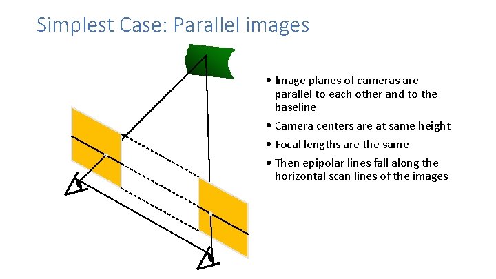
Simplest Case: Parallel images • Image planes of cameras are parallel to each other and to the baseline • Camera centers are at same height • Focal lengths are the same • Then epipolar lines fall along the horizontal scan lines of the images

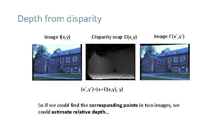
Depth from disparity image I(x, y) Disparity map D(x, y) image I´(x´, y´)=(x+D(x, y) So if we could find the corresponding points in two images, we could estimate relative depth…

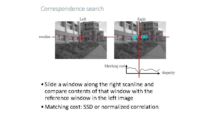
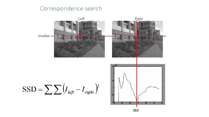
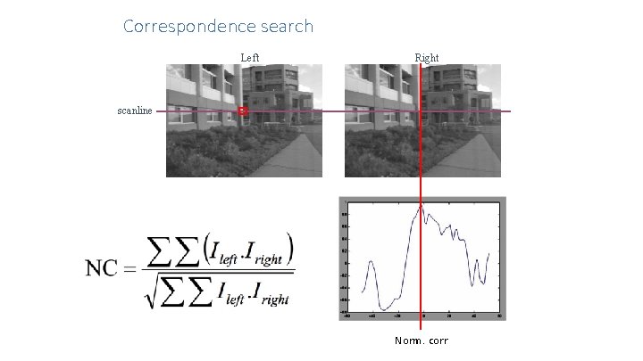
Correspondence search Left Right scanline Matching cost disparity • Slide a window along the right scanline and compare contents of that window with the reference window in the left image • Matching cost: SSD or normalized correlation

Correspondence search Left Right scanline SSD

Correspondence search Left Right scanline Norm. corr

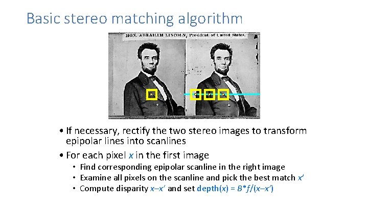
Basic stereo matching algorithm • If necessary, rectify the two stereo images to transform epipolar lines into scanlines • For each pixel x in the first image • Find corresponding epipolar scanline in the right image • Examine all pixels on the scanline and pick the best match x’ • Compute disparity x–x’ and set depth(x) = B*f/(x–x’)

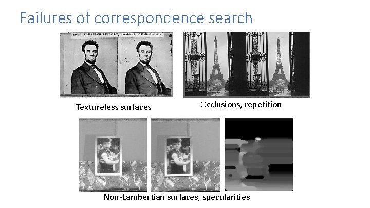
Failures of correspondence search Textureless surfaces Occlusions, repetition Non-Lambertian surfaces, specularities

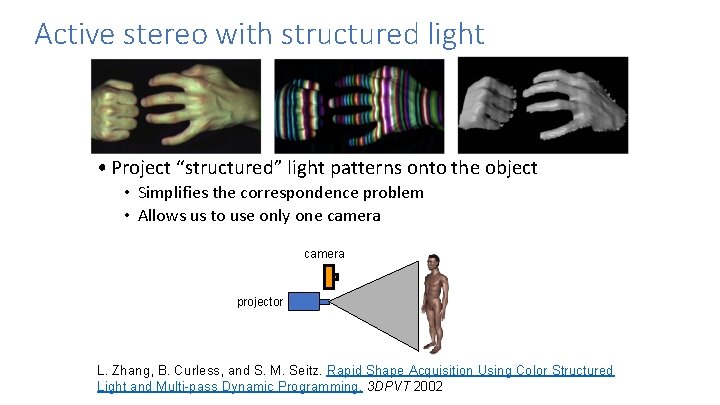
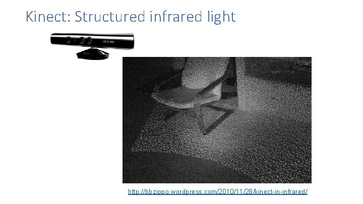
Active stereo with structured light • Project “structured” light patterns onto the object • Simplifies the correspondence problem • Allows us to use only one camera projector L. Zhang, B. Curless, and S. M. Seitz. Rapid Shape Acquisition Using Color Structured Light and Multi-pass Dynamic Programming. 3 DPVT 2002

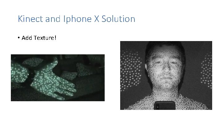
Kinect and Iphone X Solution • Add Texture!

Kinect: Structured infrared light http: //bbzippo. wordpress. com/2010/11/28/kinect-in-infrared/

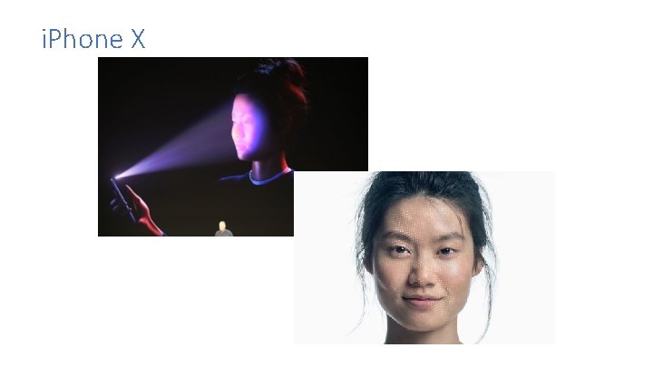
i. Phone X

Basic stereo matching algorithm • If necessary, rectify the two stereo images to transform epipolar lines into scanlines • For each pixel x in the first image • Find corresponding epipolar scanline in the right image • Examine all pixels on the scanline and pick the best match x’ • Compute disparity x–x’ and set depth(x) = B*f/(x–x’)

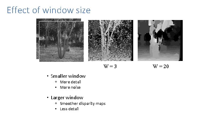
Effect of window size W=3 • Smaller window + More detail • More noise • Larger window + Smoother disparity maps • Less detail W = 20

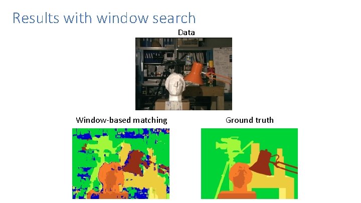
Results with window search Data Window-based matching Ground truth

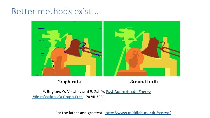
Better methods exist. . . Graph cuts Ground truth Y. Boykov, O. Veksler, and R. Zabih, Fast Approximate Energy Minimization via Graph Cuts, PAMI 2001 For the latest and greatest: http: //www. middlebury. edu/stereo/

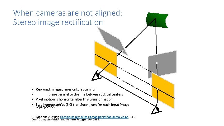
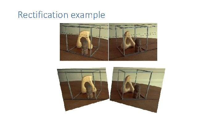
When cameras are not aligned: Stereo image rectification • Reproject image planes onto a common • plane parallel to the line between optical centers • Pixel motion is horizontal after this transformation • Two homographies (3 x 3 transform), one for each input image reprojection • C. Loop and Z. Zhang. Computing Rectifying Homographies for Stereo Vision. IEEE Conf. Computer Vision and Pattern Recognition, 1999.

Rectification example

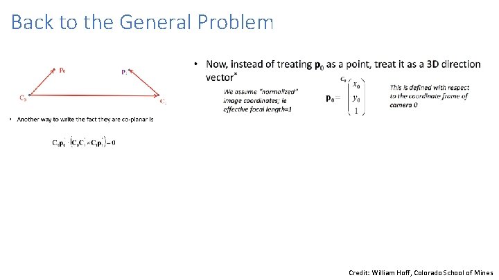
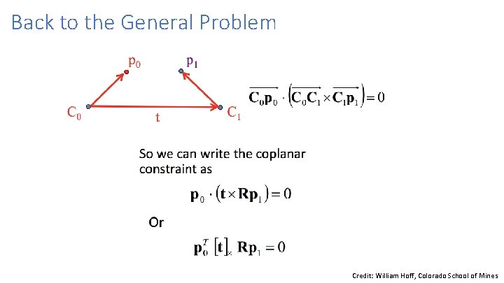
Back to the General Problem Credit: William Hoff, Colorado School of Mines

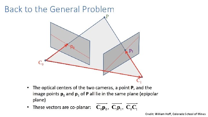
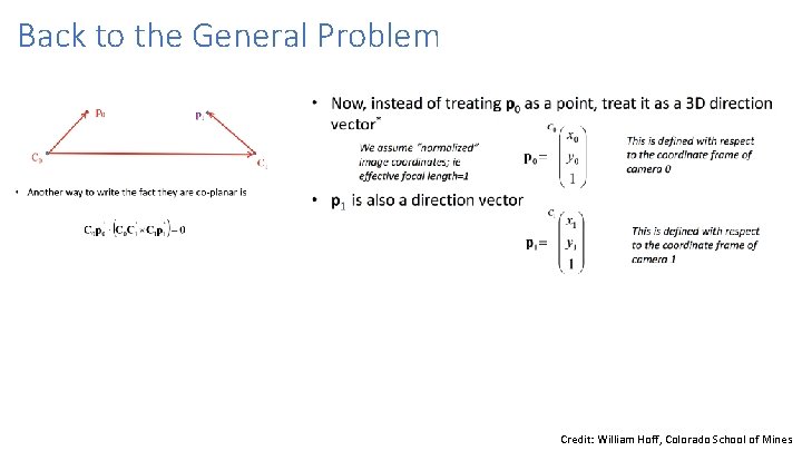
Back to the General Problem Credit: William Hoff, Colorado School of Mines

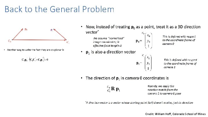
Back to the General Problem Credit: William Hoff, Colorado School of Mines

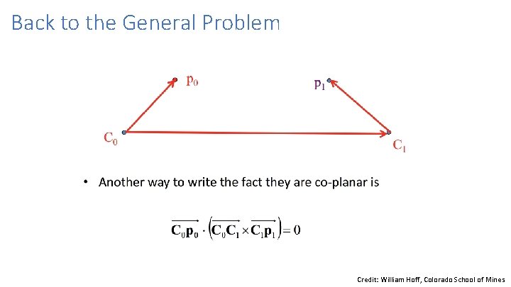
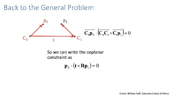
Back to the General Problem Credit: William Hoff, Colorado School of Mines

Back to the General Problem Credit: William Hoff, Colorado School of Mines

Back to the General Problem Credit: William Hoff, Colorado School of Mines

Back to the General Problem Credit: William Hoff, Colorado School of Mines

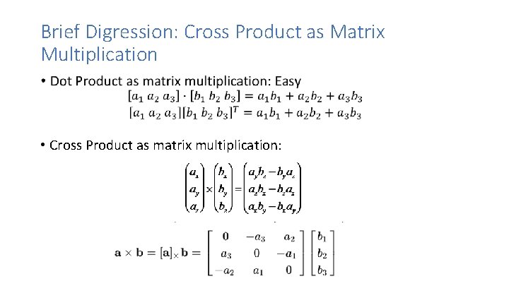
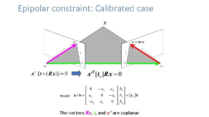
Brief Digression: Cross Product as Matrix Multiplication • • Cross Product as matrix multiplication:

Back to the General Problem Credit: William Hoff, Colorado School of Mines

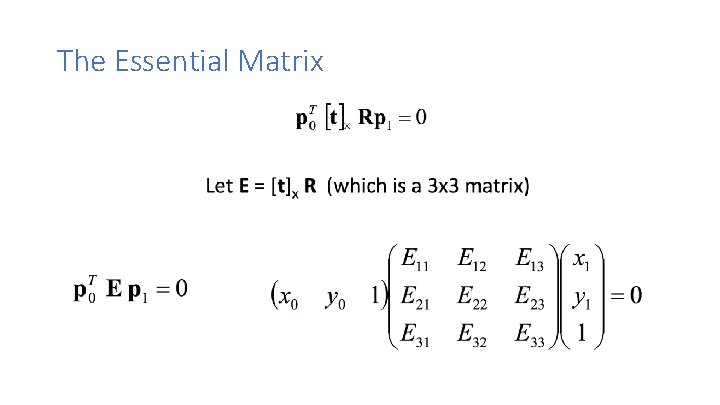
The Essential Matrix

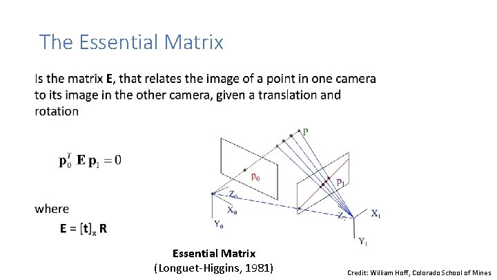
The Essential Matrix (Longuet-Higgins, 1981) Credit: William Hoff, Colorado School of Mines

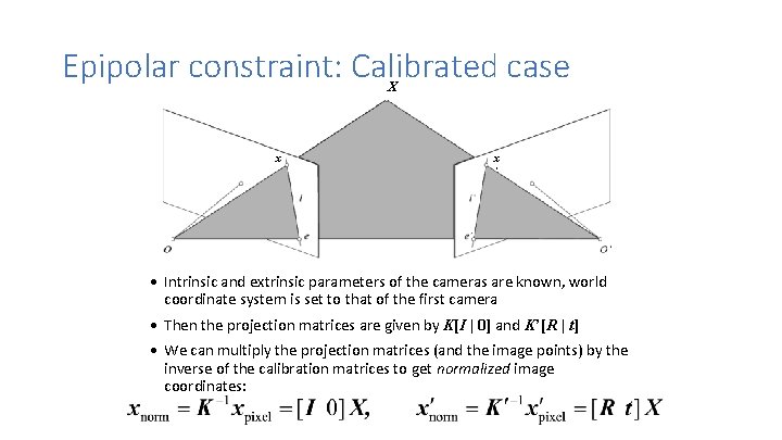
Epipolar constraint: Calibrated case X x x ’ • Intrinsic and extrinsic parameters of the cameras are known, world coordinate system is set to that of the first camera • Then the projection matrices are given by K[I | 0] and K’[R | t] • We can multiply the projection matrices (and the image points) by the inverse of the calibration matrices to get normalized image coordinates:

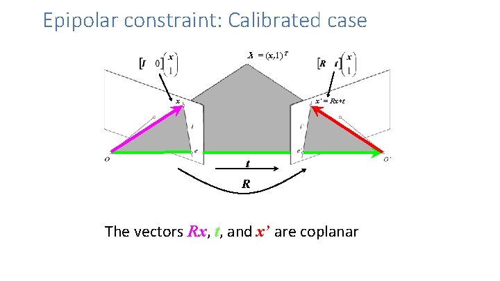
Epipolar constraint: Calibrated case X = (x, 1)T x x’ = Rx+t t R The vectors Rx, t, and x’ are coplanar

Epipolar constraint: Calibrated case X x x’ = Rx+t Recall: The vectors Rx, t, and x’ are coplanar

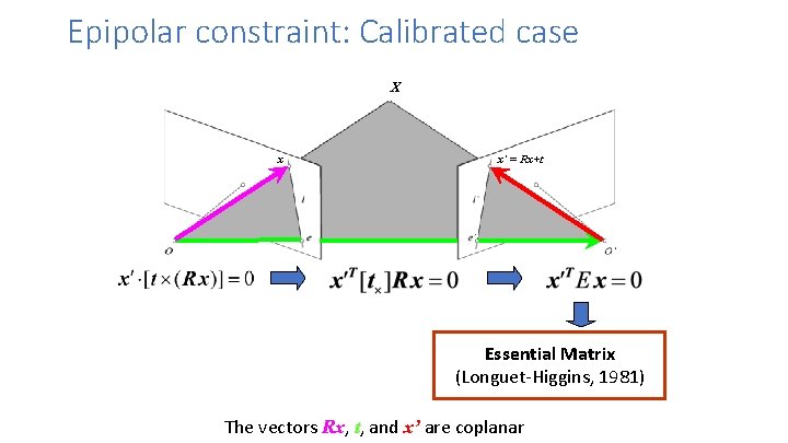
Epipolar constraint: Calibrated case X x x’ = Rx+t Essential Matrix (Longuet-Higgins, 1981) The vectors Rx, t, and x’ are coplanar

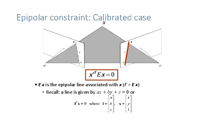
Epipolar constraint: Calibrated case X x x ’ • E x is the epipolar line associated with x (l' = E x) • Recall: a line is given by ax + by + c = 0 or

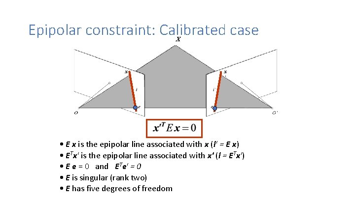
Epipolar constraint: Calibrated case X x x ’ • E x is the epipolar line associated with x (l' = E x) • ETx' is the epipolar line associated with x' (l = ETx') • E e = 0 and ETe' = 0 • E is singular (rank two) • E has five degrees of freedom

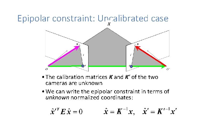
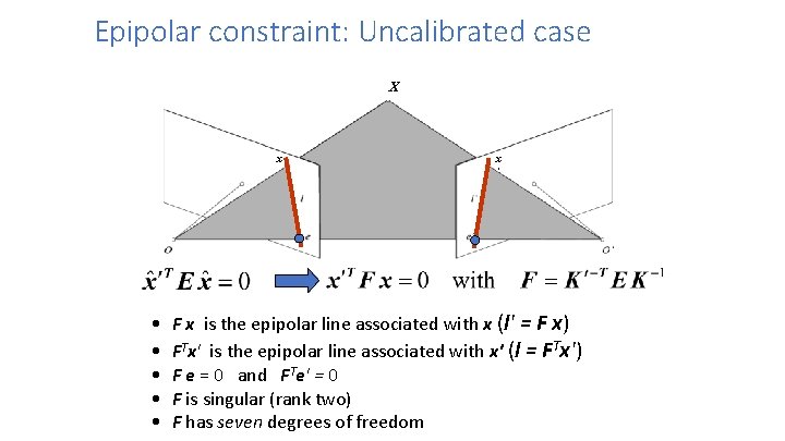
Epipolar constraint: Uncalibrated case X x x ’ • The calibration matrices K and K’ of the two cameras are unknown • We can write the epipolar constraint in terms of unknown normalized coordinates:

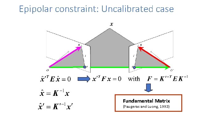
Epipolar constraint: Uncalibrated case X x x ’ Fundamental Matrix (Faugeras and Luong, 1992)

Epipolar constraint: Uncalibrated case X x • • • x ’ F x is the epipolar line associated with x (l' = F x) FTx' is the epipolar line associated with x' (l = FTx') F e = 0 and FTe' = 0 F is singular (rank two) F has seven degrees of freedom

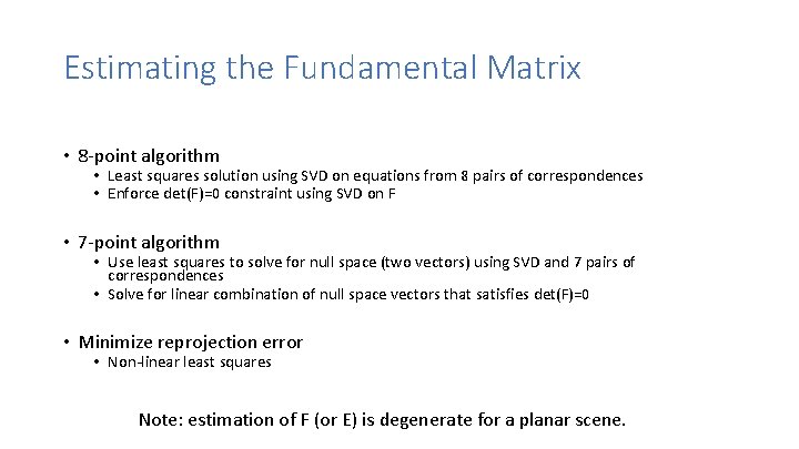
Estimating the Fundamental Matrix • 8 -point algorithm • Least squares solution using SVD on equations from 8 pairs of correspondences • Enforce det(F)=0 constraint using SVD on F • 7 -point algorithm • Use least squares to solve for null space (two vectors) using SVD and 7 pairs of correspondences • Solve for linear combination of null space vectors that satisfies det(F)=0 • Minimize reprojection error • Non-linear least squares Note: estimation of F (or E) is degenerate for a planar scene.

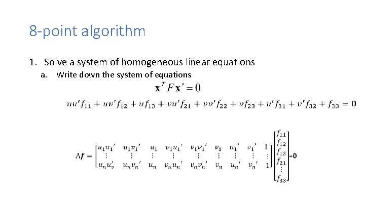
8 -point algorithm 1. Solve a system of homogeneous linear equations a. Write down the system of equations

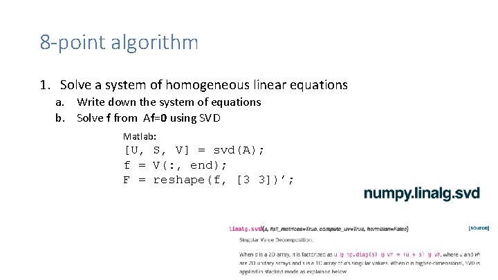
8 -point algorithm 1. Solve a system of homogeneous linear equations a. Write down the system of equations b. Solve f from Af=0 using SVD Matlab: [U, S, V] = svd(A); f = V(: , end); F = reshape(f, [3 3])’;

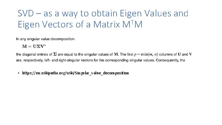
SVD – as a way to obtain Eigen Values and Eigen Vectors of a Matrix MTM • https: //en. wikipedia. org/wiki/Singular_value_decomposition

Questions? https: //www. robots. ox. ac. uk/~vgg/hz book/hzbook 2/HZepipolar. pdf 52