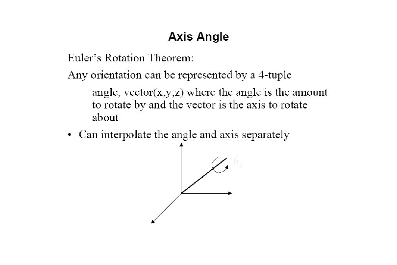
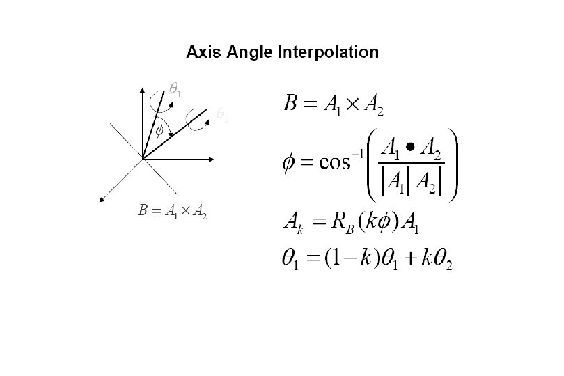
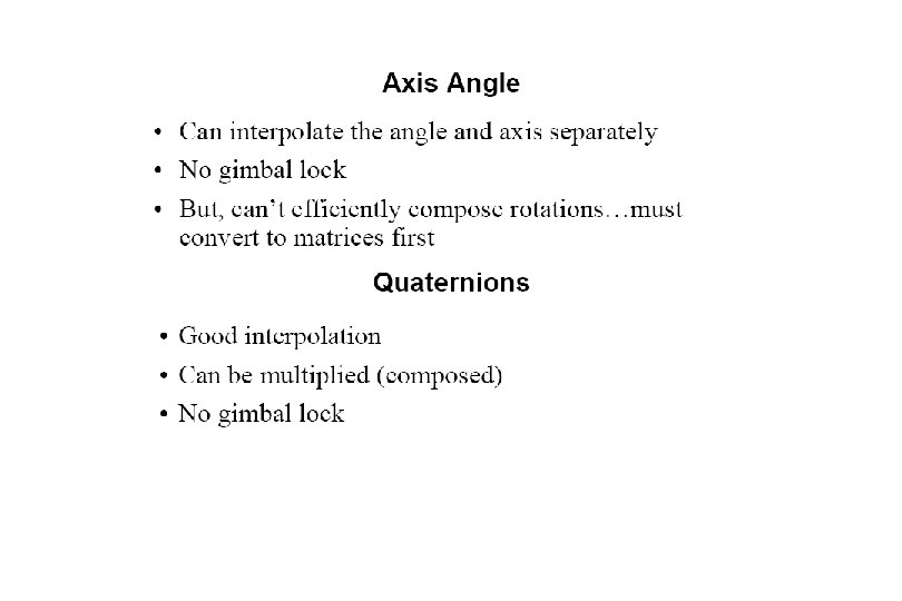
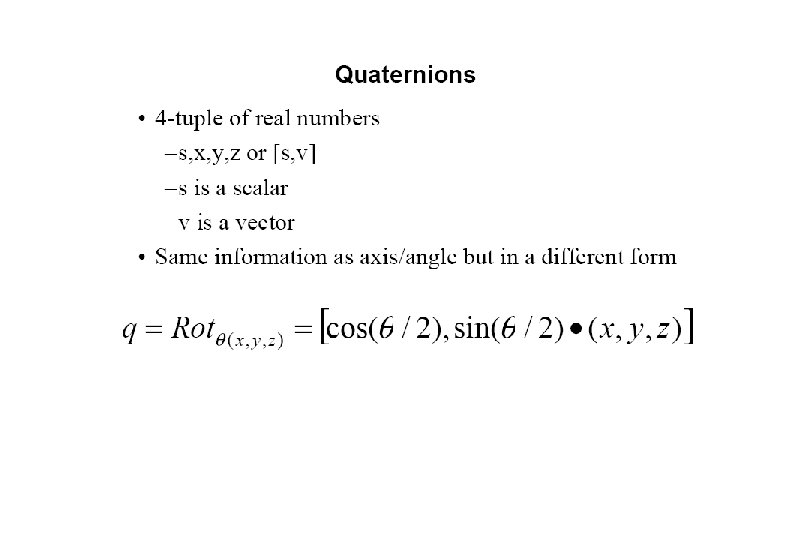
CS 445 645 Introduction to Computer Graphics Lecture


 Control Points • A set of points that influence the curve’s")

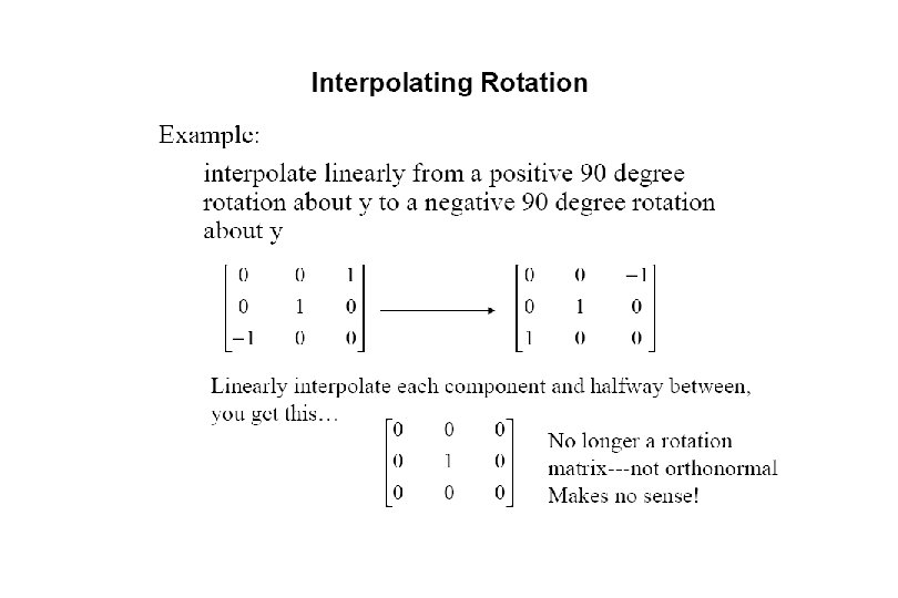
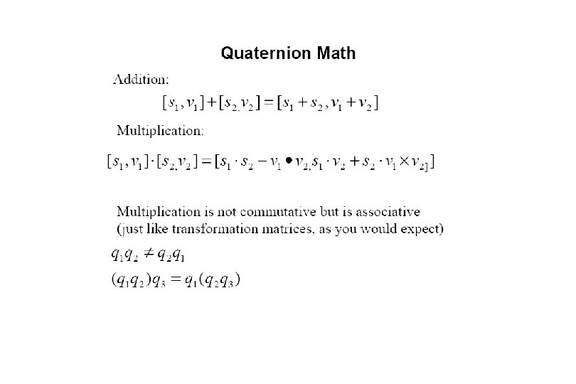
 = axt 3 + bxt 2 + cxt + dx •")

 • C 2 is 2")


![Coefficients So how do we select the coefficients? • [ax bx cx dx] and](https://slidetodoc.com/presentation_image_h/9ab4d6fc737d7dc70e09d8c323db72a9/image-33.jpg "Coefficients So how do we select the coefficients? • [ax bx cx dx] and")
 = axt 3 + bxt 2")


 position at t = 0, p")
 position at t = 1, p")

 derivative at t = 0, dp/dt")
 derivative at t = 1, dp/dt")


 to draw curves")


 defined")
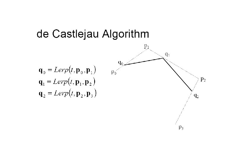

 Start with a sequence of control points Select four from")


 The native geometry element in Maya Models are composed of")


 Method Subdivision Methods")


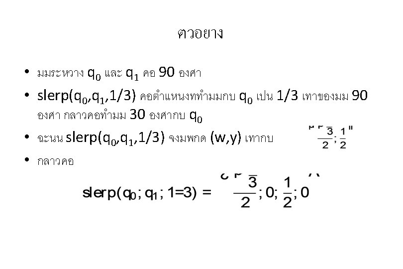
 1/3 q 0 w")
- Slides: 128
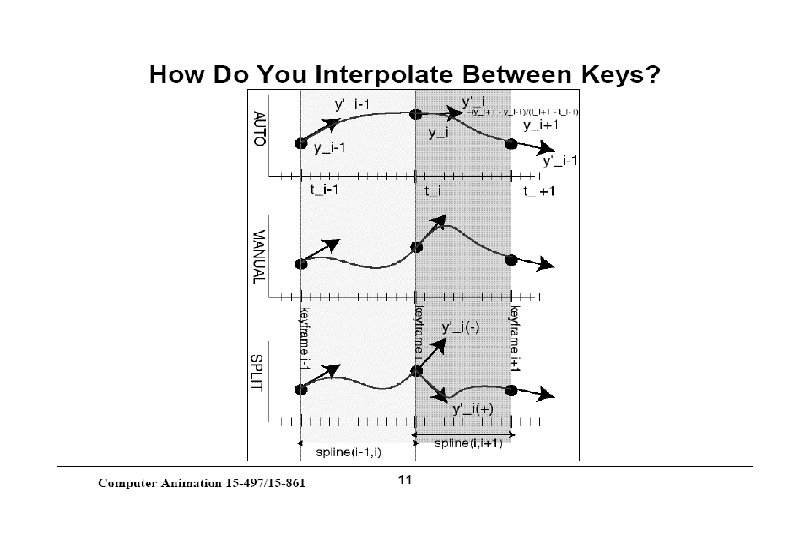
CS 445 / 645 Introduction to Computer Graphics Lecture 22 Hermite Splines
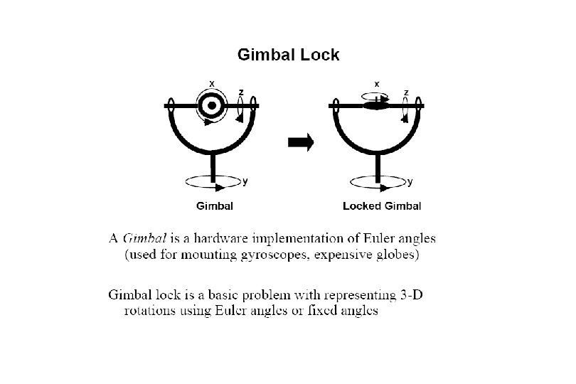
Splines – Old School Duck Spline
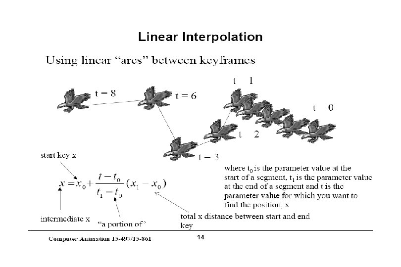
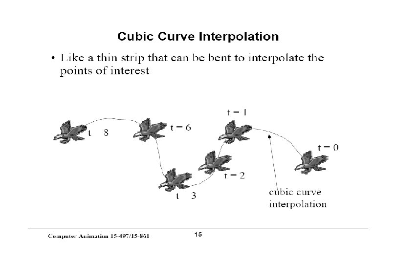
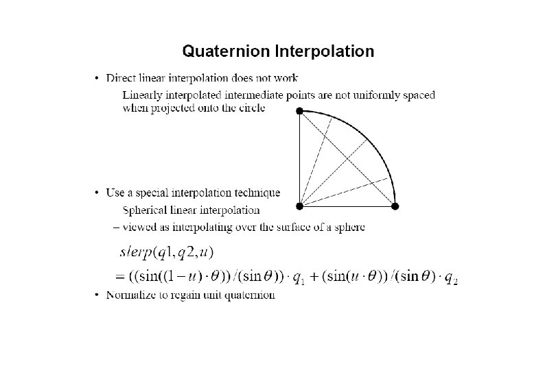
Representations of Curves Use a sequence of points… • Piecewise linear - does not accurately model a smooth line • Tedious to create list of points • Expensive to manipulate curve because all points must be repositioned Instead, model curve as piecewise-polynomial • x = x(t), y = y(t), z = z(t) – where x(), y(), z() are polynomials
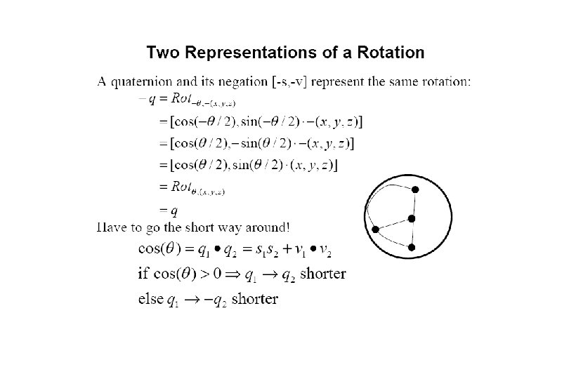
Specifying Curves (hyperlink) Control Points • A set of points that influence the curve’s shape Knots • Control points that lie on the curve Interpolating Splines • Curves that pass through the control points (knots) Approximating Splines • Control points merely influence shape
Parametric Curves Very flexible representation They are not required to be functions • They can be multivalued with respect to any dimension
Cubic Polynomials x(t) = axt 3 + bxt 2 + cxt + dx • Similarly for y(t) and z(t) Let t: (0 <= t <= 1) Let T = [t 3 t 2 t 1] Coefficient Matrix C Curve: Q(t) = T*C
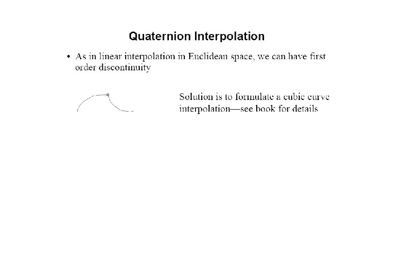
Piecewise Curve Segments One curve constructed by connecting many smaller segments end-to-end • Must have rules for how the segments are joined Continuity describes the joint • Parametric continuity • Geometric continuity
Parametric Continuity • C 1 is tangent continuity (velocity) • C 2 is 2 nd derivative continuity (acceleration) • Matching direction and magnitude of dn / dtn § Cn continous
Geometric Continuity If positions match • G 0 geometric continuity If direction (but not necessarily magnitude) of tangent matches • G 1 geometric continuity • The tangent value at the end of one curve is proportional to the tangent value of the beginning of the next curve
Parametric Cubic Curves In order to assure C 2 continuity, curves must be of at least degree 3 Here is the parametric definition of a cubic (degree 3) spline in two dimensions How do we extend it to three dimensions?
Parametric Cubic Splines Can represent this as a matrix too
Coefficients So how do we select the coefficients? • [ax bx cx dx] and [ay by cy dy] must satisfy the constraints defined by the knots and the continuity conditions
Parametric Curves Difficult to conceptualize curve as x(t) = axt 3 + bxt 2 + cxt + dx (artists don’t think in terms of coefficients of cubics) Instead, define curve as weighted combination of 4 welldefined cubic polynomials (wait a second! Artists don’t think this way either!) Each curve type defines different cubic polynomials and weighting schemes
Parametric Curves Hermite – two endpoints and two endpoint tangent vectors Bezier - two endpoints and two other points that define the endpoint tangent vectors Splines – four control points • C 1 and C 2 continuity at the join points • Come close to their control points, but not guaranteed to touch them Examples of Splines
Hermite Cubic Splines An example of knot and continuity constraints
Hermite Cubic Splines One cubic curve for each dimension A curve constrained to x/y-plane has two curves:
Hermite Cubic Splines A 2 -D Hermite Cubic Spline is defined by eight parameters: a, b, c, d, e, f, g, h How do we convert the intuitive endpoint constraints into these (relatively) unintuitive eight parameters? We know: • (x, y) position at t = 0, p 1 • (x, y) position at t = 1, p 2 • (x, y) derivative at t = 0, dp/dt • (x, y) derivative at t = 1, dp/dt
Hermite Cubic Spline We know: • (x, y) position at t = 0, p 1
Hermite Cubic Spline We know: • (x, y) position at t = 1, p 2
Hermite Cubic Splines So far we have four equations, but we have eight unknowns Use the derivatives
Hermite Cubic Spline We know: • (x, y) derivative at t = 0, dp/dt
Hermite Cubic Spline We know: • (x, y) derivative at t = 1, dp/dt
Hermite Specification Matrix equation for Hermite Curve t 3 t 2 t 1 t 0 p 1 t=0 p 2 t=1 r p 1 t=0 r p 2 t=1
Solve Hermite Matrix
Spline and Geometry Matrices MHermite GHermite
Resulting Hermite Spline Equation
Sample Hermite Curves
Blending Functions By multiplying first two matrices in lower-left equation, you have four functions of ‘t’ that blend the four control parameters These are blending functions
Hermite Blending Functions If you plot the blending functions on the parameter ‘t’
Hermite Blending Functions Remember, each blending function reflects influence of P 1, P 2, DP 1, DP 2 on spline’s shape
CS 445 / 645 Introduction to Computer Graphics Lecture 23 Bézier Curves
Splines - History Draftsman use ‘ducks’ and strips of wood (splines) to draw curves Wood splines have secondorder continuity A Duck (weight) And pass through the control points Ducks trace out curve
Bézier Curves Similar to Hermite, but more intuitive definition of endpoint derivatives Four control points, two of which are knots
Bézier Curves The derivative values of the Bezier Curve at the knots are dependent on the adjacent points The scalar 3 was selected just for this curve
Bézier vs. Hermite We can write our Bezier in terms of Hermite • Note this is just matrix form of previous equations
Bézier vs. Hermite Now substitute this in for previous Hermite MBezier
Bézier Basis and Geometry Matrices Matrix Form But why is MBezier a good basis matrix?
Bézier Blending Functions Look at the blending functions This family of polynomials is called order-3 Bernstein Polynomials • C(3, k) tk (1 -t)3 -k; 0<= k <= 3 • They are all positive in interval [0, 1] • Their sum is equal to 1
Bézier Blending Functions Thus, every point on curve is linear combination of the control points The weights of the combination are all positive The sum of the weights is 1 Therefore, the curve is a convex combination of the control points
Convex combination of control points Will always remain within bounding region (convex hull) defined by control points
Why more spline slides? Bezier and Hermite splines have global influence • One could create a Bezier curve that required 15 points to define the curve… – Moving any one control point would affect the entire curve • Piecewise Bezier or Hermite don’t suffer from this, but they don’t enforce derivative continuity at join points B-splines consist of curve segments whose polynomial coefficients depend on just a few control points • Local control Examples of Splines
B-Spline Curve (cubic periodic) Start with a sequence of control points Select four from middle of sequence (pi-2, pi-1, pi+1) d • Bezier and Hermite goes between pi-2 and pi+1 • B-Spline doesn’t interpolate (touch) any of them but approximates going through pi-1 and pi p 1 Q 4 t 4 Q 3 p 0 t 3 p 2 p 6 Q 5 t 5 p 3 t 6 Q 6 p 4 p 5 t 7
Uniform B-Splines Approximating Splines Approximates n+1 control points • P 0, P 1, …, Pn, n ¸ 3 Curve consists of n – 2 cubic polynomial segments • Q 3, Q 4, … Q n t varies along B-spline as Qi: ti <= t < ti+1 ti (i = integer) are knot points that join segment Qi to Qi+1 Curve is uniform because knots are spaced at equal intervals of parameter, t
Uniform B-Splines First curve segment, Q 3, is defined by first four control points Last curve segment, Qm, is defined by last four control points, Pm-3, Pm-2, Pm-1, Pm Each control point affects four curve segments
B-spline Basis Matrix Formulate 16 equations to solve the 16 unknowns The 16 equations enforce the C 0, C 1, and C 2 continuity between adjoining segments, Q
B-Spline Points along B-Spline are computed just as with Bezier Curves
B-Spline By far the most popular spline used C 0, C 1, and C 2 continuous
Nonuniform, Rational B-Splines (NURBS) The native geometry element in Maya Models are composed of surfaces defined by NURBS, not polygons NURBS are smooth NURBS require effort to make non-smooth
Converting Between Splines Consider two spline basis formulations for two spline types
Converting Between Splines We can transform the control points from one spline basis to another
Converting Between Splines With this conversion, we can convert a B-Spline into a Bezier Splines are easy to render
Rendering Splines Horner’s Method Incremental (Forward Difference) Method Subdivision Methods
Horner’s Method Three multiplications Three additions
Forward Difference But this still is expensive to compute • Solve for change at k (Dk) and change at k+1 (Dk+1) • Boot strap with initial values for x 0, D 0, and D 1 • Compute x 3 by adding x 0 + D 1
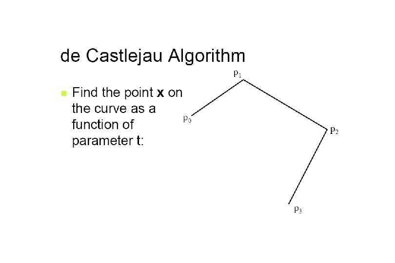
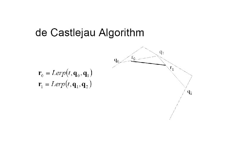
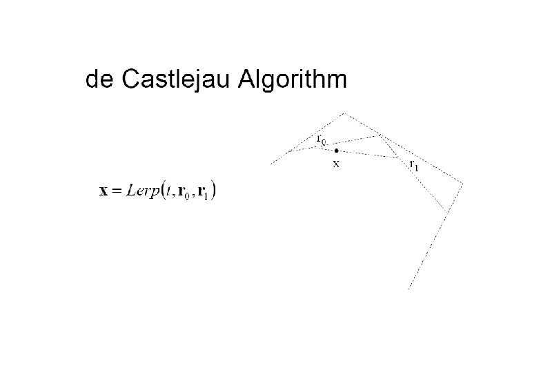
Subdivision Methods Bezier
Rendering Bezier Spline public void spline(Control. Point p 0, Control. Point p 1, Control. Point p 2, Control. Point p 3, int pix) { float len = Control. Point. dist(p 0, p 1) + Control. Point. dist(p 1, p 2) + Control. Point. dist(p 2, p 3); float chord = Control. Point. dist(p 0, p 3); if (Math. abs(len - chord) < 0. 25 f) return; fat. Pixel(pix, p 0. y); Control. Point p 11 = Control. Point. midpoint(p 0, p 1); Control. Point tmp = Control. Point. midpoint(p 1, p 2); Control. Point p 12 = Control. Point. midpoint(p 11, tmp); Control. Point p 22 = Control. Point. midpoint(p 2, p 3); Control. Point p 21 = Control. Point. midpoint(p 22, tmp); Control. Point p 20 = Control. Point. midpoint(p 12, p 21); spline(p 20, p 12, p 11, p 0, pix); spline(p 3, p 22, p 21, p 20, pix); }
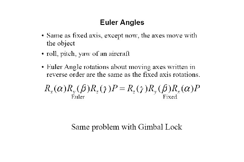
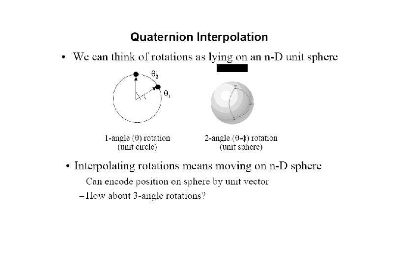
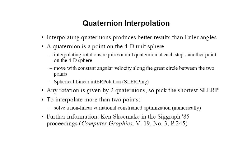
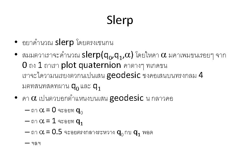
Slerp
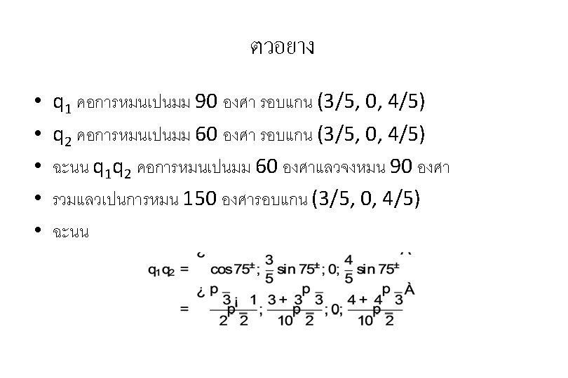
ตวอยาง y q 1 2/3 slerp(q 0, q 1, 1/3) 1/3 q 0 w