CS 4433 Database Systems Indexing Why Do We

CS 4433 Database Systems Indexing
 from")
Why Do We Learn This? ■ Find out the desired information (by value) from the database (very) quickly! – E. g. , author catalog in library ■ Indexing – Common properties of indexes – B+ trees – KD-trees – Others. . 2
 item that")
What is Indexing? • A “labeled” pointer to an (a collection of) item that satisfies some common property • Examples in the Real World? 3
 item that")
What is Indexing? • A “labeled” pointer to an (a collection of) item that satisfies some common property • Examples in the Real World? 4
 item that")
What is Indexing? • A “labeled” pointer to an (a collection of) item that satisfies some common property • Examples in the Real World? 5

Theoretically, Indexes is … ■ An index on a file speeds up selections on the search key attributes(s) ■ Search key = any subset of the attributes of a relation – attributes used to look up records in a file. – Search key is not the same as key (minimal set of attributes that uniquely identify a tuple (record) in a relation) ■ An index file consists of records (called index entries) – Entries in an index: (K, R), where: ■ K: the search key ■ R: pointers of the record OR record ids ■ Index files are typically much smaller than the original file 6

Types of Indexes ■ Ordered/Hash – Ordered indices: index entries are stored sorted on the search key value. E. g. , author catalog in library. – Hash indices: index entries are distributed uniformly across “buckets” based on search key using a “hash function”. ■ Clustered/Unclustered – Clustered = records sorted in the key order – Unclustered = no ■ Dense/sparse – Dense = Index record appears for every search-key value in the file. – Sparse = only some records have ■ Primary/secondary – Primary = on the primary key – Secondary = on any key – ■ ■ ■ Always dense Tell us the current locations of records Some textbooks interpret these differently B+ tree / Hash table / … 7

Clustered, Dense Index ■ Clustered: File is sorted on the index attribute ■ Dense: sequence of (key, pointer) pairs 10 10 20 20 30 40 50 60 70 80 8

Clustered, Dense Index index on ID attribute of instructor relation
 ■ Dense index on dept_name, with instructor file sorted")
Dense Index Files (Cont. ) ■ Dense index on dept_name, with instructor file sorted on dept_name

Clustered, Sparse Index ■ Sparse index: contains index records for only some search-key values e. g. – one key per data block – Applicable when records are sequentially ordered on search-key – Save more space – Sacrifice efficiency 10 10 30 20 50 70 30 40 90 110 130 150 50 60 70 80 11

Sparse Index Files ■ To locate a record with search-key value K we: – Find index record with largest search-key value < K – Search file sequentially starting at the record to which the index record points
 ■ Compared to dense indices: – Less space and")
Sparse Index Files (Cont. ) ■ Compared to dense indices: – Less space and less maintenance overhead for insertions and deletions. – Generally slower than dense index for locating records. ■ Good tradeoff: sparse index with an index entry for every block in file, corresponding to least search-key value in the block.

Clustered Index with Duplicate Keys ■ Dense index: point to the first record with that key 10 10 20 10 30 40 10 20 50 60 70 80 20 20 30 40 14

Unclustered Indexes ■ Often for indexing other attributes than primary key – Secondary Indexes ■ Always dense (why ? ) – The locality of values has been broken! 10 20 10 30 20 20 30 30 30 10 20 10 30 17
 (Data file) Data Records")
Clustered vs. Unclustered Index entries Data Records CLUSTERED (Index File) (Data file) Data Records UNCLUSTERED 18

Indirect Buckets for Secondary index ■ To avoid repeating keys in secondary index, use a level of indirection, called Buckets. ■ The index maintains only one keypointer pair for each search key : – The pointer for goes to a position in the bucket which contains pointers to records with search key till the next position pointed by the index

Secondary Indices Example Secondary index on salary field of instructor ■ Index record points to a bucket that contains pointers to all the actual records with that particular search-key value. ■ Secondary indices have to be dense

Primary and Secondary Indices ■ Indices offer substantial benefits when searching for records. ■ BUT: Updating indices imposes overhead on database modification --when a file is modified, every index on the file must be updated, ■ Sequential scan using primary index is efficient, but a sequential scan using a secondary index is expensive – Each record access may fetch a new block from disk – Block fetch requires about 5 to 10 milliseconds, versus about 100 nanoseconds for memory access

Problems ■ the growth of the size of the database, indices also grow. – need to keep the index records in the main memory so as to speed up the search operations. – a large size index cannot be kept in memory which leads to multiple disk accesses. – Binary searching requires too many seeks ■ Searching for a key on a disk often involves seeking to different disk tracks ■ It can be very expensive to keep the index in sorted order – If inserting a key involves moving a large number of other keys in the index, index maintenance is very nearly impractical on secondary storage for indexes with large numbers of keys – We need to find a way to make insertions and deletions to indexes that will not require massive reorganization

Multilevel Index ■ helps in breaking down the index into several smaller indices in order to make the outermost level so small – it can be saved in a single disk block, which can easily be accommodated anywhere in the main memory. ■ We need data structures that allow efficient insertion and deletion i. e. are good in dynamic situations

B+ Trees ■ B+ Tree Intuition: – Give up sequentiality of index and Try to get “balance” by dynamic reorganization – automatically reorganizes itself with small, local, changes, in the face of insertions and deletions. – Reorganization of entire file is not required to maintain performance. – (Minor) disadvantage of B+-trees: ■ extra insertion and deletion overhead, space overhead. 24
 ■ Each node has")
B+-Tree Node Structure ■ Parameter d = the degree (order) ■ Each node has [d, 2 d] keys (except root) ■ Each interior node that is not a root or a leaf has pointer to [d+1, 2 d+1] children. ■ A leaf node has pointers [d+1, 2 d+1] to record ■ Typical Node K 1 p 1 [X , K 1) – – ■ K 2 p 2 [K 1, K 2) K 3 p 4 [K 2, K 3) [K 3, Y) Ki are the search-key values Pi are pointers to children (for non-leaf nodes) or pointers to records or buckets of records (for leaf nodes). The search-keys in a node are ordered K 1 < K 2 < K 3 <. . . < Kn– 1 (Initially assume no duplicate keys, address duplicates later)
 120 [30, 120) 240")
B+ Trees Basics – Internal node: 30 [X , 30) 120 [30, 120) 240 [120, 240) [240, Y) – Leaf: 40 40 50 50 60 next leaf 60 26
 A B+-tree is a rooted tree satisfying the following")
B+-Tree Index Files (Cont. ) A B+-tree is a rooted tree satisfying the following properties: ■ It is a balanced tree – All paths from root to leaf are of the same length ■ Special cases: – If the root is not a leaf, it has at least 2 children. – If the root is a leaf (that is, there are no other nodes in the tree), it can have between 0 and (2 d– 1) values ■ Each node should fit in a block

+ Example of B -Tree

Searching a B+ Tree ■ Point queries with exact key values: – Start at the root – Proceed down, to the leaf ■ Range queries: – As above – Then sequential traversal on leafs Select name From people Where age = 25 Select name From people Where 20 <= age and age <= 30 29
")
B+ Tree Example Select name From person Where age = 30 (Where age >=30) (Where 20<=age and age <=30) Root (d=1) d=2 80 20 10 10 15 15 18 60 100 20 18 20 30 30 40 40 50 60 65 120 140 80 65 80 85 85 90 90 30

B+ Tree Design ■ Each block will have space for 2 d search key and 2 d+1 pointers. ■ Pick n as large as possible that fits into a block ■ Example 14. 10 ■ Example: – Key size = 4 bytes – Pointer size = 8 bytes – Block size = 4096 byes ■ How large is d? ■ 2 d x 4 + (2 d+1) x 8 <= 4096 ■ So, d = 170 31

B+ Trees in Practice ■ Typical order: 100. Typical fill-factor: 67%. – average fan-out = 133 ■ Typical capacities: – Height 4: 1334 = 312, 900, 700 records – Height 3: 1333 = 2, 352, 637 records ■ Can often hold top levels in buffer pool: – Level 1 = 1 page = 8 Kbytes – Level 2 = 133 pages = 1 Mbyte – Level 3 = 17, 689 pages = 133 MBytes 32
: Find leaf where K belongs,")
Insertion in a B+ Tree ■ Insert (K, P): Find leaf where K belongs, insert – If no overflow (2 d keys or less), halt – If overflow (2 d+1 keys), split node, insert the middle key into parent: ■ Example: d=2 insert(K 5, P 4) K 1 P 0 K 2 P 1 K 3 P 2 K 4 P 3 P 4 (K 3, K 1 P 0 K 2 P 1 K 3 P 2 K 4 P 3 P 4 K 5 p 5 K 1 P 0 K 2 P 1 ) to parent K 4 P 2 P 3 K 5 P 4 p 5 – If leaf, keep K 3 too in right node – When root splits, new root has 1 key only ■ that’s why root is special for degree satisfaction 33
: Find leaf where K belongs,")
Deletion in a B+ Tree ■ Delete (K, P): Find leaf where K belongs, delete – If that leaf has d or more key, halt – If less than d, rebalance ■ Rotate ■ merge K 1 P 0 K 4 K 2 P 3 P 1 ■ Example: d=2 delete (K 4) K 1 P 0 K 2 P 1 k 3 p 2 k 4 p 3 K 5 P 4 P 1 K 1 P 0 K 2 P 1 K 5 P 4 k 3 p 3 K 5 P 4 34

Insertion in a B+ Tree Insert K=19 80 20 10 10 15 15 18 60 100 20 18 20 30 30 40 40 50 60 65 120 140 80 65 80 85 85 90 90 35

Insertion in a B+ Tree After Insertion 80 20 10 10 15 15 18 60 19 18 19 100 20 30 40 40 50 60 65 120 140 80 65 80 85 85 90 90 36

Insertion in a B+ Tree Now Insert K=25 80 20 10 10 15 15 18 60 19 18 19 100 20 30 40 40 50 60 65 120 140 80 65 80 85 85 90 90 37

Insertion in a B+ Tree After Insertion 80 20 10 10 15 15 18 60 19 18 19 100 20 25 30 30 40 40 50 60 120 65 140 80 65 80 85 85 90 90 38

Insertion in a B+ Tree Now Split 80 20 10 10 15 15 18 60 19 18 19 100 20 25 30 30 40 40 50 60 120 65 140 80 65 80 85 85 90 90 39

Insertion in a B+ Tree After the Split 80 20 10 10 15 15 18 19 30 60 20 25 100 30 30 40 40 50 120 60 50 60 140 65 80 85 85 90 90 40

Deletion from a B+ Tree Delete 30 80 20 10 10 15 15 18 19 30 60 20 25 100 30 30 40 40 50 120 60 50 60 140 65 80 85 85 90 90 41

Deletion from a B+ Tree After Deleting 30 80 May change to 40, or not 20 10 10 15 15 18 19 30 60 20 25 100 40 40 50 120 60 50 60 140 65 80 85 85 90 90 42

Deletion from a B+ Tree Delete 25 80 20 10 10 15 15 18 19 30 60 20 25 100 40 40 50 120 60 50 60 140 65 80 85 85 90 90 43

Deletion from a B+ Tree After deleting 25, Need to rebalance: Rotate 80 20 10 10 15 15 18 19 18 30 60 100 20 19 20 40 40 50 120 60 50 60 140 65 80 85 85 90 90 44

Deletion from a B+ Tree Now Delete 40 80 19 10 10 15 15 18 30 19 18 19 20 60 100 20 40 40 50 120 60 50 60 140 65 80 85 85 90 90 45

Deletion from a B+ Tree After deleting 40, Rotation not possible. Need to merge nodes 80 19 10 10 15 15 18 30 19 18 19 20 20 60 100 50 120 60 50 60 140 65 80 85 85 90 90 46

Deletion from a B+ Tree Final Tree 80 19 10 10 15 15 18 60 19 18 19 20 20 100 50 120 60 50 60 140 65 80 85 85 90 90 47

Inverted Index ■ Boolean retrieval – Queries on unstructured text data – arguably the simplest model to base an information retrieval system on – Primary commercial retrieval tool for 3 decades – queries are Boolean expressions, ■ e. g. , get the document that contains the words “CAESAR AND BRUTUS”? – the search engine returns all documents that satisfy the Boolean expression – How? 48

1 - Term-document Incidence Matrix • Entry is 1 if term occurs. • Example: CALPURNIA occurs in Julius Caesar. • Entry is 0 if term doesn’t occur. • Example: CALPURNIA doesn’t occur in The tempest. 49

Incidence Vectors ■ So we have a 0/1 vector for each term ■ To answer the query BRUTUS AND CAESAR AND NOT CALPURNIA 1. Take the vectors for BRUTUS, CAESAR and CALPURNIA 2. Complement the vector of CALPURNIA 3. Do a (bitwise) and on the three vectors ■ 110100 AND 110111 AND 101111 = 100100 50

2 -Inverted Index ■ Problem for the incidence matrix : – extremely large – extremely sparse – What is a better representations? ■ We only record the 1 s ■ Inverted Index – For each term t, we store a list of all documents (ids) that contain t 51 dictionary postings

Inverted index construction 1. Collect the documents to be indexed 2. Tokenize the text, turning each document into a list of tokens 3. Do linguistic preprocessing, producing a list of normalized tokens, which are the indexing terms: 4. Index the documents that each term occurs in by creating an inverted index, consisting of a dictionary and postings 52

Processing Boolean queries ■ Consider the query: BRUTUS AND CALPURNIA, to find all matching documents using inverted index: 1. Locate BRUTUS in the dictionary 2. Retrieve its postings list from the postings file 3. Locate CALPURNIA in the dictionary 4. Retrieve its postings list from the postings file 5. Intersect the two postings lists 6. Return intersection to user 53

Query Optimization ■ Consider a query with n terms, n > 2 – For each of the terms, get its postings list, then intersect them together – What is the best order for processing this query? ■ Example query: BRUTUS AND CALPURNIA AND CAESAR – Simple and effective optimization: Process in order of increasing frequency 54 ■ Start with the shortest postings list, then keep cutting further ■ In this example, first CAESAR, then CALPURNIA, then BRUTUS

Multidimensional Indexes ■ When we see attributes of relations as coordinates, a database stores a point set in higher dimensions ■ Indexing with multiple keys – Spatial databases and Geographic information system (GIS) – Multimedia databases – Medical applications ■ The queries to be supported: – partial-match queries: specify values for a subset of the dimensions – range queries: give the range for each dimension – nearest-neighbor queries: ask for the closest point to the given point 55

Example SQL Query: Select * From Customers Where 3 K<Salary<4 K AND 2<Children<4 AND 25<Age<40 25 56 40
 – Jon Bentley, 1975, author of Programming Pearls")
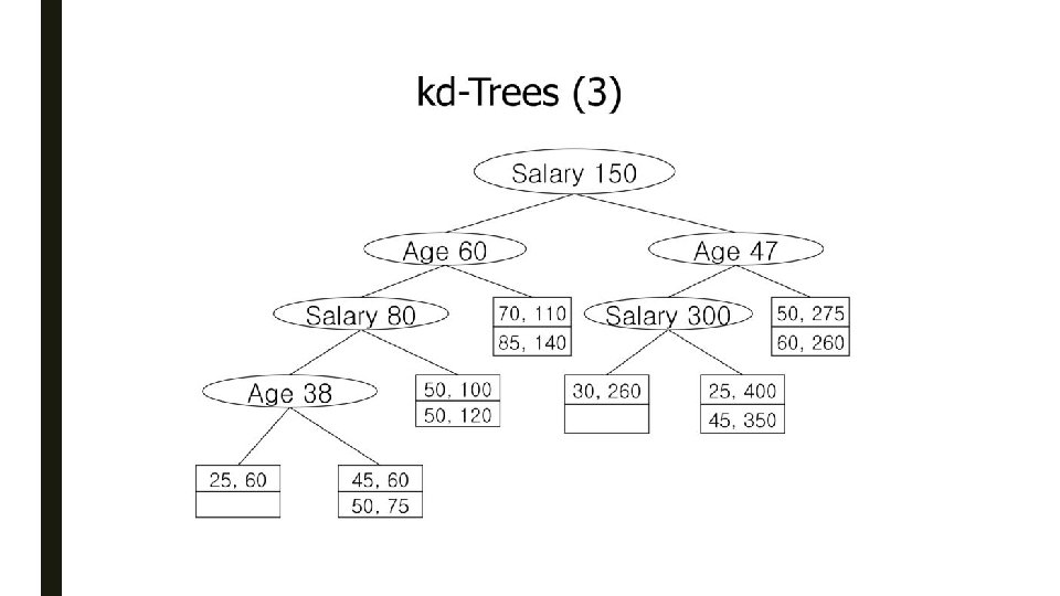
KD-Tree ■ kd-Tree (k-dimensional search tree) – Jon Bentley, 1975, author of Programming Pearls – Idea: Split the point set alternatingly by x-coordinate and by y-coordinate 1. split by x-coordinate: split by a vertical line that has half the points left and half right 2. split by y-coordinate: split by a horizontal line that has half the points below and half above ■ Interior nodes will only have an attribute, a dividing value for that attribute and pointers to left and right children ■ Leaves will be blocks with space for as many records as a block can hold 57

KD-Tree: Example 58

KD-Tree Construction Algorithm 60

Range Queries in KD-Tree 61

KD-Tree Querying Algorithm 62

Higher Dimensions ■ A 3 -dimensional kd-tree alternates splits on x-, y-, and z-coordinate – A 3 D range query is performed with a box ■ Query Processing – Intersection of B and region(v) depends on intersection of facets of B analyze by axes-parallel planes 63

Quad Trees ■ Quad trees are space-partition trees whose nodes are associated with squares – Raphael Finkel and Jon Bentley in 1974 – If a node is not a leaf, its square is partitioned into four equal-sized squares associated with its children 64

Quad Trees ■ The square associated with the root contains all points in point set P – Recursive splitting is continued until there is at most one (or k) point left in a square – Demo: https: //google. github. io/closurelibrary/source/closure/goog/demos/quadtree. html 65
 Tree – A tree data structure mainly used")
R Tree ■ R (Range, Rectangle) Tree – A tree data structure mainly used for spatial access methods, i. e. , for indexing multidimensional information such as geographical coordinates, rectangles or polygons – Generalization of B+ trees to higher dimensions ■ A height balanced tree like the B+ Tree – – R-tree represents data objects in intervals (MBR, minimum bounding rectangle) in several dimensions ■ Exact-point and range lookups! – – 66 B+ tree: balanced hierarchy of 1 -d ranges Show me all Pizza places within 2 miles of MSCS building Antonin Guttman in 1984

R Tree Structure K R 1 A R 3 L R 2 G B D R 4 H R 5 E R 6 I F R 1 R 2 R 3 R 4 M : maximum number of entries m : minimum number of entries (>= M/2) (1)Every node contains between m and M index records unless it is the root. (2) Each leaf node has the smallest rectangle that spatially contains the n-dimensional data objects. (3)Each non-leaf node has the smallest rectangle that spatially contains the rectangles in the child node. (4) The root node has at least two children unless it is a leaf. (5) All leaves appear on the same level. <MBR, Pointer to a child node> R 5 R 6 <MBR, Pointer to a spatial object> A B 67 D E F G H I K L

R Tree Search K R 1 A L R 2 R 3 G B H R 5 E S R 6 I D R 4 F R 1 R 2 R 3 R 4 A B 68 R 5 R 6 D E F G H I K L Query: Find all objects whose rectangles are overlapped with a search rectangle S 1. Start at root and locate all child nodes which intersect S (via linear search). 2. Search the subtrees of those child nodes. 3. When you get to the leaves, return entries whose rectangles intersect S. Searches may require inspecting several paths. – Worst case running time is not so good.

R Tree Search K R 1 A L R 2 R 3 G B H R 5 E S R 6 I D R 4 F R 1 R 2 R 3 R 4 A B 69 R 5 R 6 D E F G H I K L

R Tree Search K R 1 A L R 2 R 3 G B H R 5 E S R 6 I D R 4 F R 1 R 2 R 3 R 4 A B 70 R 5 R 6 D E F G H I K L

R Tree Search K R 1 A L R 2 R 3 G B H R 5 E S R 6 I D R 4 F R 1 R 2 R 3 R 4 A B 71 R 5 R 6 D E F G H I K L

R Tree Search K R 1 A L R 2 R 3 G B H R 5 E S R 6 I D R 4 F R 1 R 2 R 3 R 4 A B 72 R 5 R 6 D E F G H I K L

R Tree Search K R 1 A L R 2 R 3 G B H R 5 E S R 6 I D R 4 F R 1 R 2 R 3 R 4 A B 73 R 5 R 6 D E F G H I K L

R Tree Search K R 1 A R 6 L R 2 R 3 B G E S D R 4 H R 5 I F R 1 R 2 R 3 R 4 A B 74 R 5 R 6 D E F G H I K L Answer: B and D overlapped objects with S

R-Tree Insertion K R 1 A B L R 2 R 3 G X R 5 E D R 4 H I F R 1 R 2 R 3 R 4 A B R 5 R 6 D E 75 F G H I R 6 K L Insert a new spatial object X Insertion is done at the leaves Where to put new entry with rectangle R? 1. Start at root. 2. Go down the tree by choosing child whose rectangle needs the least enlargement to include R. In case of a tie, choose child with smallest area. 3. If there is room in the correct leaf node, insert it. Otherwise split the node (to be continued. . . ) 4. Adjust the tree. . . 5. If the root was split into nodes N 1 and N 2, create new root with N 1 and N 2 as children.

R-Tree Insertion K R 1 A B L R 2 R 3 G X R 5 E D R 4 H I F R 1 R 2 R 3 R 4 A B 76 R 5 R 6 D E F G H I R 6 K L Find the proper child node - least enlargement - smallest MBR if child nodes contains a new object

R-Tree Insertion R 2 K L R 1 A R 3 B G X R 5 E D R 4 H I F R 1 R 2 R 3 R 4 A B 77 R 5 R 6 D E F R 6 G H I K L

R-Tree Insertion K R 3 B R 1 A L R 2 G X R 5 E D R 4 H I F R 1 R 2 R 3 R 4 A B 78 R 5 R 6 D E F G H I R 6 K L

R-Tree Insertion K R 1 A B L R 2 R 3 G X R 5 E R 4 H I D F R 1 R 2 R 3 R 4 A B 79 R 5 R 6 D E F G H I R 6 K L

R-Tree Insertion K R 3 R 1 A B L R 2 G X R 5 E D R 4 H I F R 1 R 2 R 3 R 4 A B 80 X R 5 R 6 D E F Empty Spot G H I R 6 K L

Splitting Nodes After Insertion ■ Problem: Divide M+1 entries among two nodes so that it is unlikely that the nodes are needlessly examined during a search.

Split After Insertion K R 3 B R 1 A R 3 H R 5 E F R 3 R 4 82 F A X G H I K L I R 1 R 2 R 3 R 4’’ A B H R 5 Y E R 6 L R 2 G R 5 R 6 D E R 1 R 4’’ D F R 4’ R 1 R 2 X B I D R 4 A B K L R 2 G X R 6 X D Y E R 5’ R 6 F G H I K L

Split ■ The bad split may cause multiple paths for searching A A B VS. E F B E F Objective: Minimize the total area of the two covering rectangles 83

Splitting Nodes After Insertion ■ Problem: Divide M+1 entries among two nodes so that it is unlikely that the nodes are needlessly examined during a search. ■ Solution: Minimize the probability of accessing the nodes during a query. 1. Exhaustive algorithm. 2. Quadratic algorithm. 3. Linear time algorithm

A Quadratic Split Algorithm ■ Split S into S 1 and S 2 1. Initial step: choose two candidates far apart most – Choose max{MBR(a, b)– area(a)– area(b)} for all a, b 2. Put a and b into different groups, S 1 and S 2 3. Iteration step: For each entry c, 1. calculate d 1=MBR(S 1, c)| and d 2=MBR(S 2, c)| where di is the area increase in covering rectangle of group Si when c is added. 2. Find c with maximum |d 1 - d 2| and add c to the group whose covering rectangle will increase the least A ■ Algorithm is quadratic in M. ■ Linear in number of dimensions B E F 85

R Tree Deletion ■ Find the entry to delete and remove it from the appropriate leaf L ■ Eliminate the node if it has too few entries (≤ m/2) – propagate node elimination upward as necessary ■ Re-insert its entries using insertion method – easier to implement – prevent gradual deterioration 86

Bitmap Index ■ A special kind of index that stores the bulk of its data as bit arrays (commonly called "bitmaps") ■ Answers most queries by performing bitwise logical operations on these bitmaps – bitwise logical operations are fast! ■ Designed for cases where number of distinct values is low, in other words, the values repeat very frequently – Index sizes are small for categorical attributes with low cardinality 87

Example ■ Suppose a file consists of records with two fields, F and G, of type integer and string, respectively. The current file has six records, numbered 1 through 6, with the following values in order: 88

Example ■ A bitmap index for the first field, F, would have three bit-vectors, each of length 6 as shown in the table – In each case, the 1's indicate in which records the corresponding value appears 89 No 30(F) 40(F) 50(F) 1 1 0 0 2 1 0 0 3 0 1 0 4 0 0 1 5 0 1 0 6 1 0 0

Example ■ A bitmap index for the second field, G, would have three bit-vectors, each of length 6 as shown in the table – In each case, the 1's indicate in which records the corresponding string appears 90 No FOO (G) BAR (G) BAZ (G) 1 1 0 0 2 0 1 0 3 0 0 1 4 1 0 0 5 0 1 0 6 0 0 1

Motivation for Bitmap Indexes ■ Bitmap indexes can help answer range queries ■ Example: – Given is the data of a jewelry stores, and the attributes considered are age and salary 91

Example ■ A bitmap index for the first field Age, would have seven bit-vectors, each of length 12 as shown in the table ■ In each case, the 1's indicate in which records the corresponding string appears 92

Example ■ A bitmap index for the second field Salary, would have ten bit-vectors, each of length 12 as shown in the table ■ In each case, the 1's indicate in which records the corresponding string appears 93

Example • 94 Suppose we want to find the jewelry buyers with an age in the range 45 -55 and a salary in the range 100 -200 • We first find the bit-vectors for the age values in this range; in this example there are only two: 010000000100 and 001110000010, for 45 and 50, respectively • If we take their bitwise OR, we have a new bit-vector with 1 in position i if and only if the ith record has an age in the desired range • This bit-vector is 011110000110

Example • Suppose we want to find the jewelry buyers with an age in the range 45 -55 and a salary in the range 100 -200 – Next, we find the bit-vectors for the salaries between 100 and 200 thousand – There are four, corresponding to salaries 100, 110, 120, and 140; their bitwise OR is 000111100000 ■ The last step is to take the bitwise AND of the two bit-vectors we calculated by OR 011110000110 (50, 100) (50, 120) AND 000111100000 -----------------000110000000 95

Hash Tables ■ Recall basics – There are n buckets – A hash function f(k) maps a key k to {0, 1, …, n-1} – Store in bucket f(k) a pointer to record with key k ■ Secondary storage: bucket = block, use overflow blocks when needed 96
 stores 2 keys + pointers –")
Hash Table Example ■ Assume 1 bucket (block) stores 2 keys + pointers – h(e)=0 – h(b)=h(f)=1 – h(g)=2 – h(a)=h(c)=3 0 1 e b f 2 g 3 a c 97
=3 – Read")
Searching in a Hash Table ■ Search for a: – Compute h(a)=3 – Read bucket 3 – 1 disk access 0 1 e b f 2 g 3 a c 98

Insertion in Hash Table ■ Place in right bucket, if there exists space – E. g. h(d)=2 0 1 e b f 2 g 3 a d c 99

Insertion in Hash Table ■ Create overflow block, if no space – E. g. h(k)=1 ■ More overflow blocks may be needed 0 1 e b k f 2 g 3 a d c 100

Hash Table Performance ■ Excellent, if no overflow blocks ■ Degrades considerably when number of keys exceeds the number of buckets (i. e. many overflow blocks) ■ Other problems: – Memory requirement – Dynamic maintenance – Equality queries only! 101

Extensible Hash Table ■ Allows hash table to grow, to avoid performance degradation ■ Assume a hash function h that returns numbers in {0, …, 2 k – 1} – Start with n = 2 i << 2 k (size of the hash table), only look at first i most significant bits – E. g. i=1, n=2, k=4 The first i bits (i = 1) i=1 0 1 0(010) 1 1(011) 1 102
 1 1(011)")
Insertion in Extensible Hash Table ■ Insert 1110 i=1 0 1 0(010) 1 1(011) 1 1(110) 103
 1")
Insertion in Extensible Hash Table ■ Now insert 1010 i=1 0 1 0(010) 1 1(011) 1 1(110), 1(010) ■ Need to extend table, split blocks – i becomes 2 so n=4 104

Insertion in Extensible Hash Table ■ n=4 ■ Now insert 1010 i=2 Doubling the hash table 00 01 10 11 0(010) 1 10(11) 2 10(10) 11(10) 2 105

Insertion in Extensible Hash Table ■ Now insert 0000, i=2 ■ then 0101 ■ Need to split block 00 01 10 11 0(010) 1 0(000), 0(101) 10(11) 2 10(10) 11(10) 2 106

Insertion in Extensible Hash Table ■ After splitting the block i=2 00 01 10 11 00(10) 2 00(00) 01(01) 2 10(10) 11(10) 2 107

Performance Extensible Hash Table ■ No overflow blocks: access always one read ■ BUT: – Extensions can be costly and disruptive – After an extension table may no longer fit in memory 108

Linear Hash Table ■ Idea: extend only one entry at a time ■ Problem: n= no longer a power of 2 ■ Let i be #bits necessary to address n buckets – 2 i-1 < n <= 2 i ■ After computing h(k), use last i bits: – If last i bits represent a number >= n, change msb from 1 to 0 (get a number < n) 109
11 – Bit flip: 11")
Linear Hash Table Example ■ i=2 N=3 – Insert (01)11 – Bit flip: 11 01 (01)00 i=2 (11)00 (01)11 BIT FLIP 00 01 10 (10)10 110
00 i=2 (10)00 (11)00 (01)11")
Linear Hash Table Example ■ Insert 1000: overflow blocks… (01)00 i=2 (10)00 (11)00 (01)11 00 01 10 (10)10 111

Linear Hash Tables ■ Extension: independent on overflow blocks ■ Extend n: =n+1 when average number of records per block exceeds (say) 80% 112

Linear Hash Table Extension ■ From n=3 to n=4 – Only need to touch one block (which one ? ) i=2 (01)00 (11)00 (01)11 00 01 10 (01)11 i=2 (10)10 00 01 10 11 (01)11 113

Linear Hash Table Extension ■ From n=3 to n=4 finished ■ Extension from n=4 to n=5 (new bit) ■ Need to touch every single block (why ? ) – Need to look last 3 bits which affect all keys (01)00 (11)00 i=2 (10)10 00 01 10 11 (01)11 114
- Slides: 112