CS 430536 Computer Graphics I Intro to Curves

CS 430/536 Computer Graphics I Intro to Curves Week 4, Lecture 7 David Breen, William Regli and Maxim Peysakhov Geometric and Intelligent Computing Laboratory Department of Computer Science Drexel University http: //gicl. cs. drexel. edu 1

Outline • • • Introduction to 2 D curves Functional representations Parametric cubic curves Introduction to Bézier curves Continuity 2

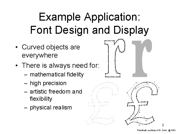
Example Application: Font Design and Display • Curved objects are everywhere • There is always need for: – mathematical fidelity – high precision – artistic freedom and flexibility – physical realism 3 Pics/Math courtesy of G. Farin @ ASU

Example Application: Graphic Design and Arts 4 Courtesy of http: //www. pilot 3 d. com

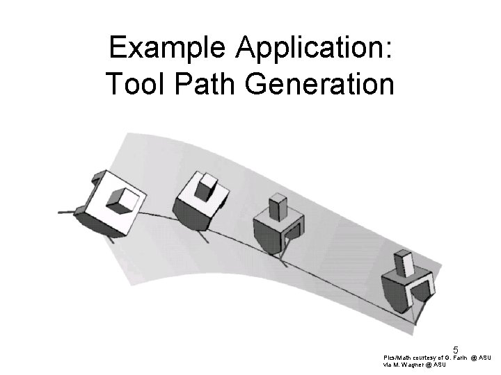
Example Application: Tool Path Generation 5 Pics/Math courtesy of G. Farin @ ASU via M. Wagner @ ASU

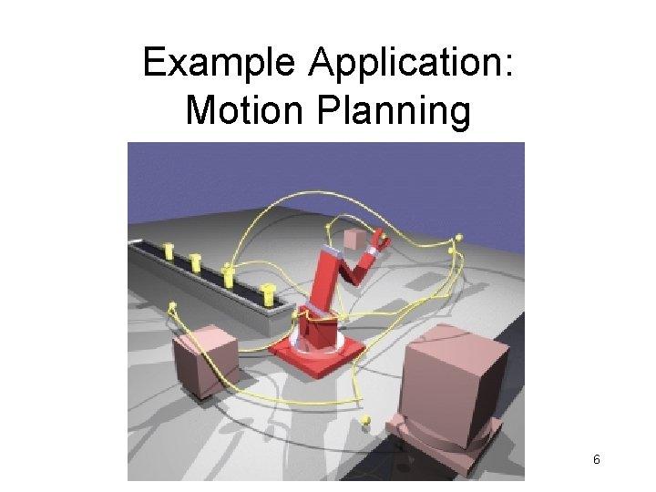
Example Application: Motion Planning 6

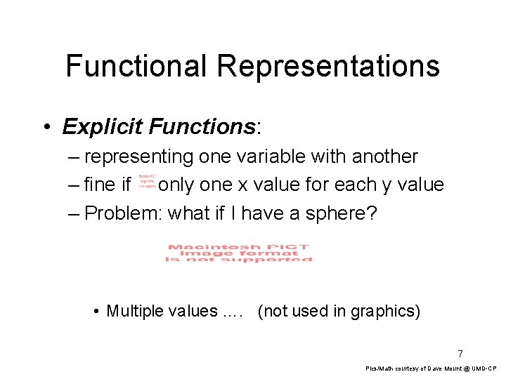
Functional Representations • Explicit Functions: – representing one variable with another – fine if only one x value for each y value – Problem: what if I have a sphere? • Multiple values …. (not used in graphics) 7 Pics/Math courtesy of Dave Mount @ UMD-CP

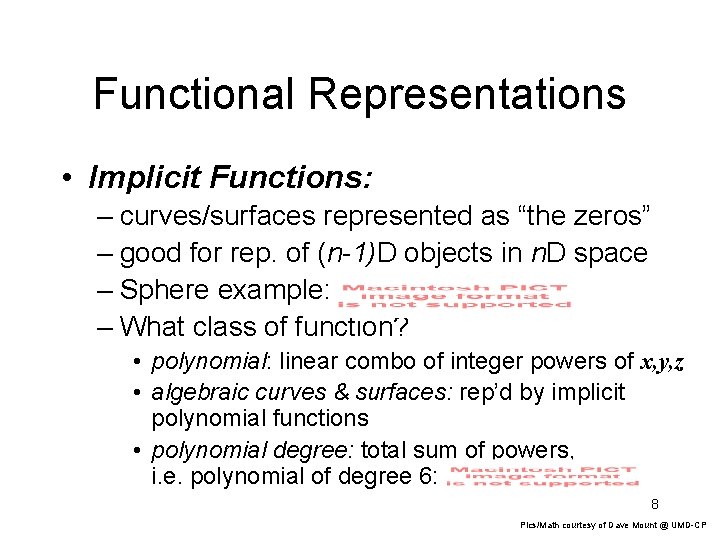
Functional Representations • Implicit Functions: – curves/surfaces represented as “the zeros” – good for rep. of (n-1)D objects in n. D space – Sphere example: – What class of function? • polynomial: linear combo of integer powers of x, y, z • algebraic curves & surfaces: rep’d by implicit polynomial functions • polynomial degree: total sum of powers, i. e. polynomial of degree 6: 8 Pics/Math courtesy of Dave Mount @ UMD-CP

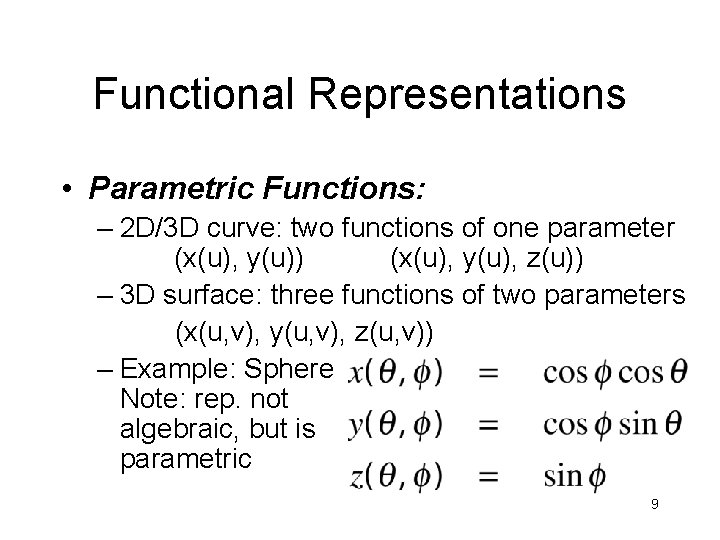
Functional Representations • Parametric Functions: – 2 D/3 D curve: two functions of one parameter (x(u), y(u)) (x(u), y(u), z(u)) – 3 D surface: three functions of two parameters (x(u, v), y(u, v), z(u, v)) – Example: Sphere Note: rep. not algebraic, but is parametric 9

Functional Representations • Which is best? ? – It depends on the application – Implicit is good for • computing ray/surface intersection • point inclusion (inside/outside test) • mass & volume properties – Parametric is good for • subdivision, faceting for rendering • Surface & area properties • popular in graphics 10

Issues in Specifying/Designing Curves/Surfaces • Note: the internal mathematical representation can be very complex – high degree polynomials – hard to see how parameters relate to shape • How do we deal with this complexity? – Use curve control points and either • Interpolate • Approximate 11

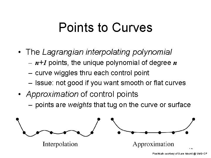
Points to Curves • The Lagrangian interpolating polynomial – n+1 points, the unique polynomial of degree n – curve wiggles thru each control point – Issue: not good if you want smooth or flat curves • Approximation of control points – points are weights that tug on the curve or surface 12 Pics/Math courtesy of Dave Mount @ UMD-CP

Warning, Warning: Pending Notation Abuse • t and u are used interchangeably as a parameterization variable for functions • Why? – t historically is “time”, certain parametric functions can describe “change over time” (e. g. motion of a camera, physics models) – u comes from the 3 D world, i. e. where two variables describe a B-spline surface • u and v are the variables for defining a surface • Choice of t or u depends on the text/reference 13

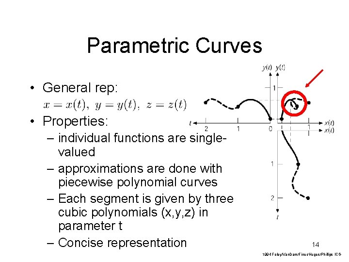
Parametric Curves • General rep: • Properties: – individual functions are singlevalued – approximations are done with piecewise polynomial curves – Each segment is given by three cubic polynomials (x, y, z) in parameter t – Concise representation 14 1994 Foley/Van. Dam/Finer/Huges/Phillips ICG

Cubic Parametric Curves • Balance between – Complexity – Control – Wiggles – Amount of computation – Non-planar 15

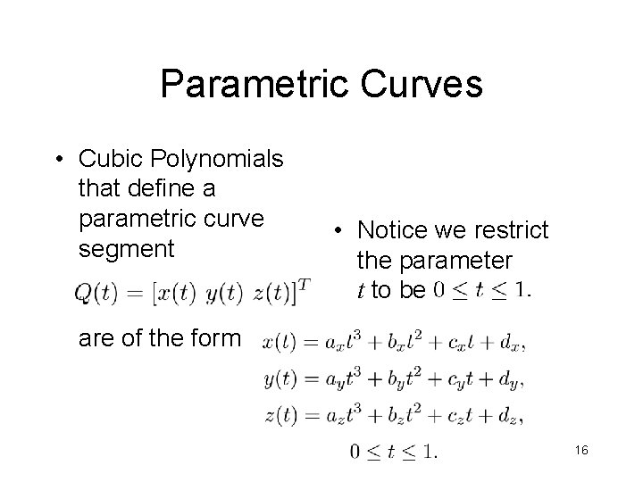
Parametric Curves • Cubic Polynomials that define a parametric curve segment • Notice we restrict the parameter t to be are of the form 16

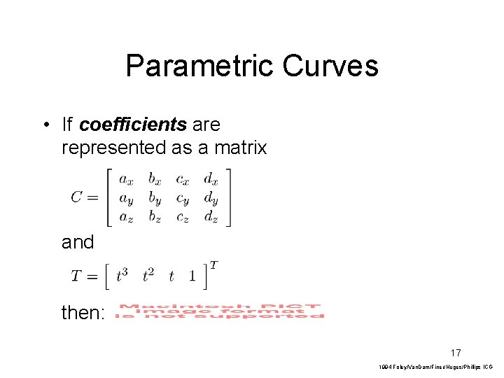
Parametric Curves • If coefficients are represented as a matrix and then: 17 1994 Foley/Van. Dam/Finer/Huges/Phillips ICG

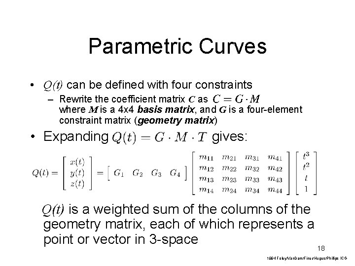
Parametric Curves • Q(t) can be defined with four constraints – Rewrite the coefficient matrix C as where M is a 4 x 4 basis matrix, and G is a four-element constraint matrix (geometry matrix) • Expanding gives: Q(t) is a weighted sum of the columns of the geometry matrix, each of which represents a point or vector in 3 -space 18 1994 Foley/Van. Dam/Finer/Huges/Phillips ICG

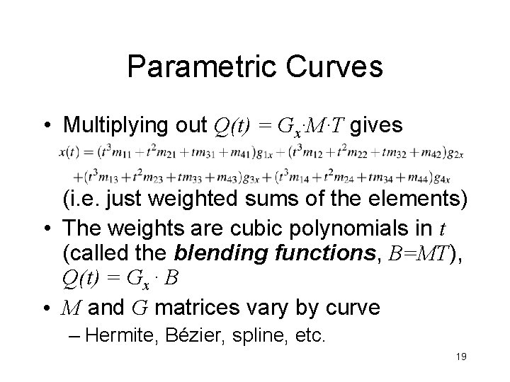
Parametric Curves • Multiplying out Q(t) = Gx·M·T gives (i. e. just weighted sums of the elements) • The weights are cubic polynomials in t (called the blending functions, B=MT), Q(t) = Gx · B • M and G matrices vary by curve – Hermite, Bézier, spline, etc. 19

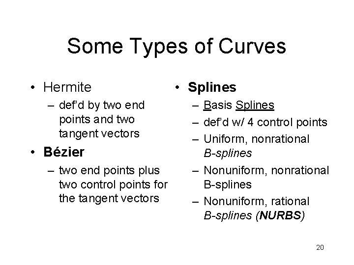
Some Types of Curves • Hermite – def’d by two end points and two tangent vectors • Bézier – two end points plus two control points for the tangent vectors • Splines – Basis Splines – def’d w/ 4 control points – Uniform, nonrational B-splines – Nonuniform, rational B-splines (NURBS) 20

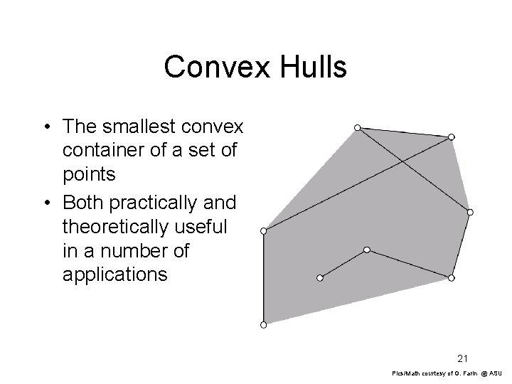
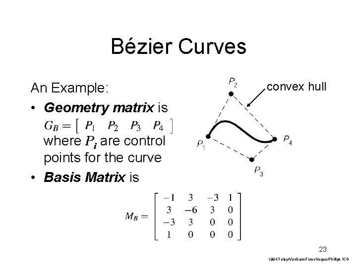
Convex Hulls • The smallest convex container of a set of points • Both practically and theoretically useful in a number of applications 21 Pics/Math courtesy of G. Farin @ ASU

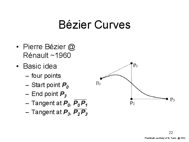
Bézier Curves • Pierre Bézier @ Rénault ~1960 • Basic idea – – – four points Start point P 0 End point P 3 Tangent at P 0, P 0 P 1 Tangent at P 3, P 2 P 3 22 Pics/Math courtesy of G. Farin @ ASU

Bézier Curves An Example: • Geometry matrix is convex hull where Pi are control points for the curve • Basis Matrix is 23 1994 Foley/Van. Dam/Finer/Huges/Phillips ICG

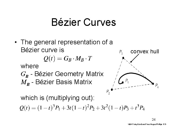
Bézier Curves • The general representation of a Bézier curve is convex hull where GB - Bézier Geometry Matrix MB - Bézier Basis Matrix which is (multiplying out): 24 1994 Foley/Van. Dam/Finer/Huges/Phillips ICG

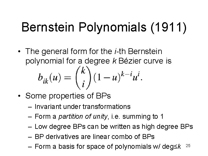
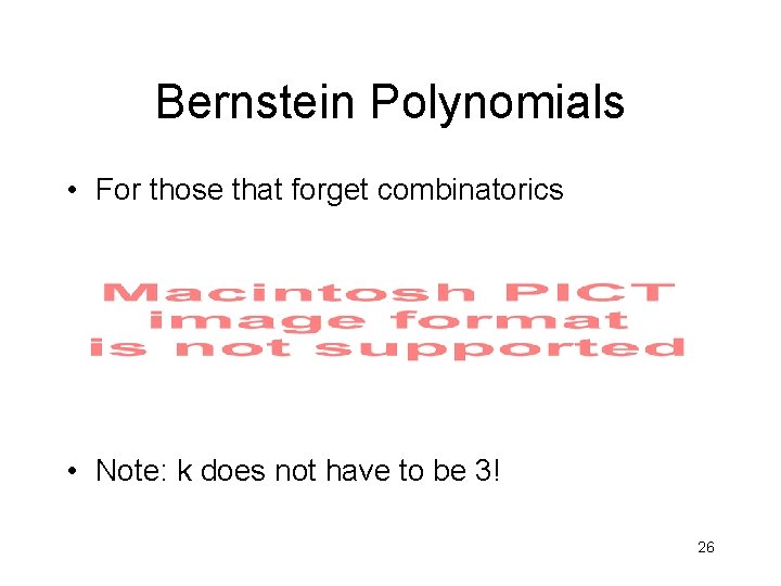
Bernstein Polynomials (1911) • The general form for the i-th Bernstein polynomial for a degree k Bézier curve is • Some properties of BPs – – – Invariant under transformations Form a partition of unity, i. e. summing to 1 Low degree BPs can be written as high degree BPs BP derivatives are linear combo of BPs Form a basis for space of polynomials w/ deg≤k 25

Bernstein Polynomials • For those that forget combinatorics • Note: k does not have to be 3! 26

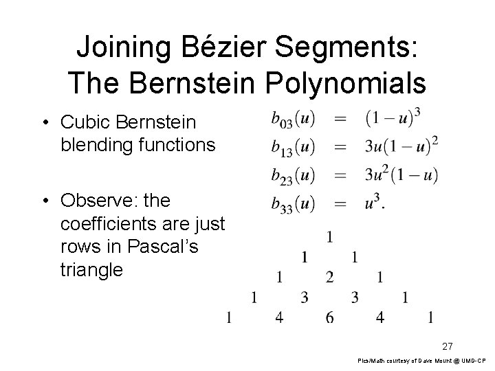
Joining Bézier Segments: The Bernstein Polynomials • Cubic Bernstein blending functions • Observe: the coefficients are just rows in Pascal’s triangle 27 Pics/Math courtesy of Dave Mount @ UMD-CP

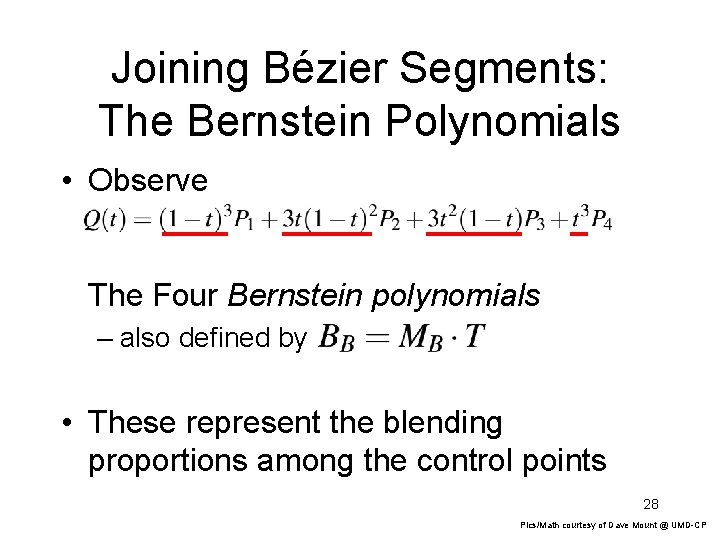
Joining Bézier Segments: The Bernstein Polynomials • Observe The Four Bernstein polynomials – also defined by • These represent the blending proportions among the control points 28 Pics/Math courtesy of Dave Mount @ UMD-CP

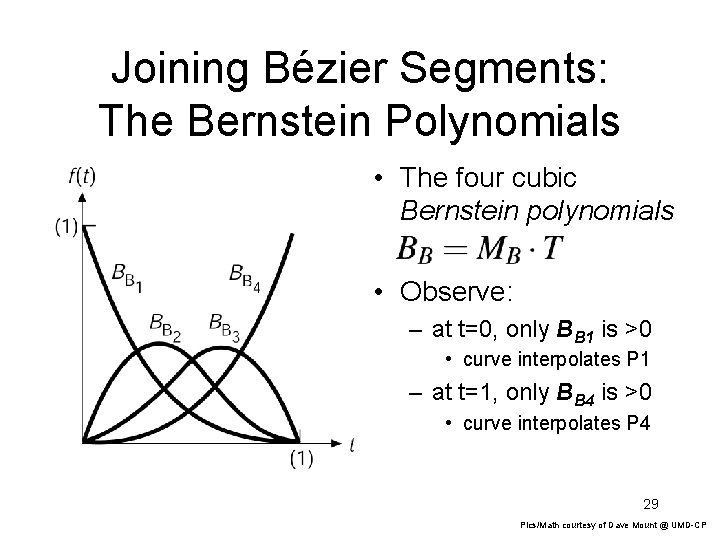
Joining Bézier Segments: The Bernstein Polynomials • The four cubic Bernstein polynomials • Observe: – at t=0, only BB 1 is >0 • curve interpolates P 1 – at t=1, only BB 4 is >0 • curve interpolates P 4 29 Pics/Math courtesy of Dave Mount @ UMD-CP

General Form of Bezier Curve 30

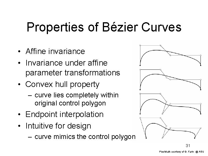
Properties of Bézier Curves • Affine invariance • Invariance under affine parameter transformations • Convex hull property – curve lies completely within original control polygon • Endpoint interpolation • Intuitive for design – curve mimics the control polygon 31 Pics/Math courtesy of G. Farin @ ASU

Issues with Bézier Curves • Creating complex curves may (with lots of wiggles) requires many control points – potentially a very high-degree polynomial • Bézier blending functions have global support over the whole curve – move just one point, change whole curve • Improved Idea: link (C 1) lots of low degree (cubic) Bézier curves end-to-end 32

Continuity Two types: • Geometric Continuity, Gi: – endpoints meet – tangent vectors’ directions are equal • Parametric Continuity, Ci: – endpoints meet – tangent vectors’ directions are equal – tangent vectors’ magnitudes are equal • In general: C implies G but not vice versa 33

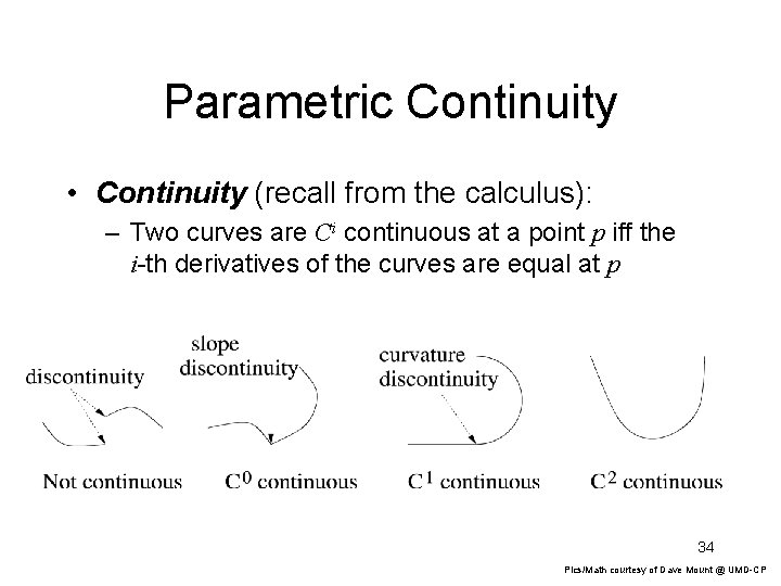
Parametric Continuity • Continuity (recall from the calculus): – Two curves are Ci continuous at a point p iff the i-th derivatives of the curves are equal at p 34 Pics/Math courtesy of Dave Mount @ UMD-CP

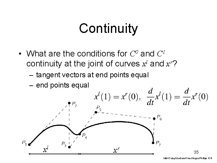
Continuity • What are the conditions for C 0 and C 1 continuity at the joint of curves xl and xr? – tangent vectors at end points equal – end points equal xl xr 35 1994 Foley/Van. Dam/Finer/Huges/Phillips ICG

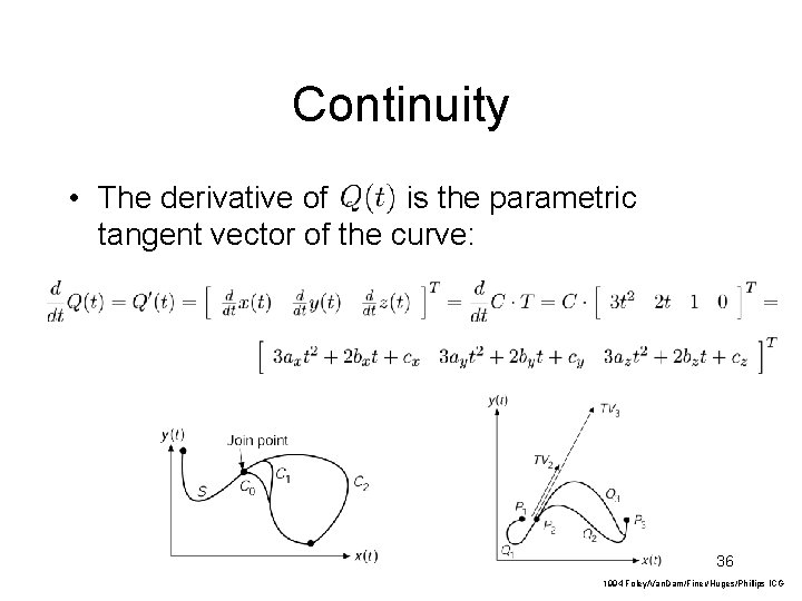
Continuity • The derivative of is the parametric tangent vector of the curve: 36 1994 Foley/Van. Dam/Finer/Huges/Phillips ICG

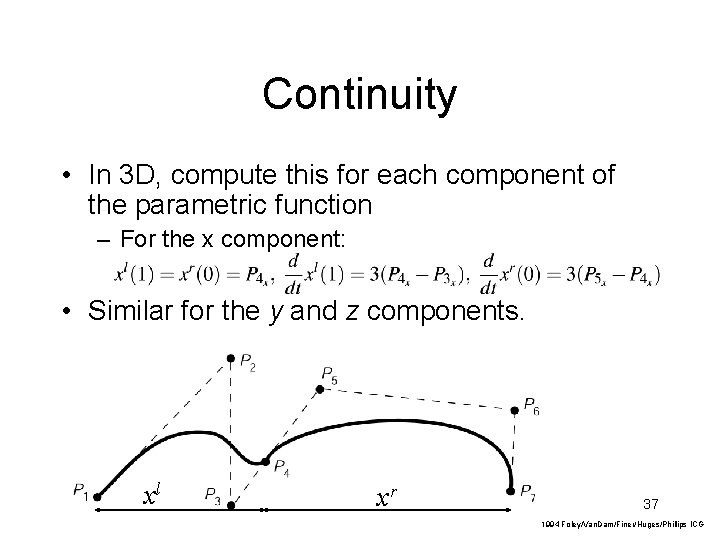
Continuity • In 3 D, compute this for each component of the parametric function – For the x component: • Similar for the y and z components. xl xr 37 1994 Foley/Van. Dam/Finer/Huges/Phillips ICG