CS 426 Game Physics Jason Leigh Electronic Visualization

CS 426 Game Physics © Jason Leigh Electronic Visualization Lab, University of Illinois at Chicago 2003 -2007 Electronic Visualization Laboratory (EVL) University of Illinois at Chicago

Application in Video Games • Racing games: Cars, snowboards, etc. . – Simulates how cars drive, collide, rebound, flip, etc. . • Sports games – Simulates trajectory of soccer, basket balls. • Increasing use in First Person Shooters: Un. Real – Used to simulate bridges falling and breaking apart when blown up. – Dead bodies as they are dragged by a limb. • Miscellaneous uses: – Flowing flags / cloth. • Problem is that real time physics is very compute intensive. But it is becoming easier with faster CPUs. Electronic Visualization Laboratory (EVL) University of Illinois at Chicago

Definitions • Kinematics – the study of movement over time. Not concerned with the cause of the movement. • Dynamics – Study of forces and masses that cause the kinematic quantities to change as time progresses. Electronic Visualization Laboratory (EVL) University of Illinois at Chicago

Particle Systems • Infinitely small objects that have Mass, Position and Velocity • They are also useful for modeling non-rigid objects such as jelly or cloth (more later). • Motion of a Newtonian particle is governed by: – F=ma (F=force, m=mass, a=acceleration) – a=dv/dt (Change of velocity over time- v=velocity; t=time) – v=dp/dt (Change of distance over time- p=distance or position) – So a basic data structure for a particle consists of: F, m, v, p. Electronic Visualization Laboratory (EVL) University of Illinois at Chicago

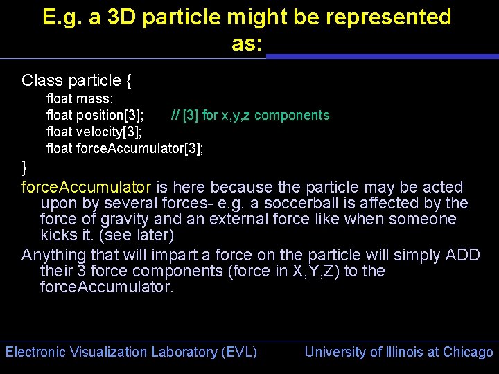
E. g. a 3 D particle might be represented as: Class particle { float mass; float position[3]; // [3] for x, y, z components float velocity[3]; float force. Accumulator[3]; } force. Accumulator is here because the particle may be acted upon by several forces- e. g. a soccerball is affected by the force of gravity and an external force like when someone kicks it. (see later) Anything that will impart a force on the particle will simply ADD their 3 force components (force in X, Y, Z) to the force. Accumulator. Electronic Visualization Laboratory (EVL) University of Illinois at Chicago

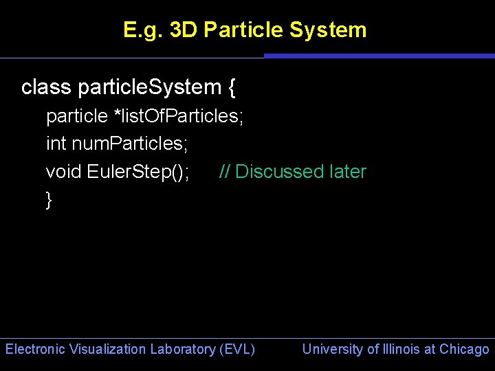
E. g. 3 D Particle System class particle. System { particle *list. Of. Particles; int num. Particles; void Euler. Step(); // Discussed later } Electronic Visualization Laboratory (EVL) University of Illinois at Chicago

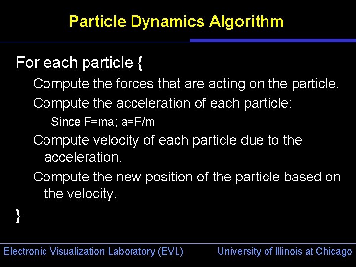
Particle Dynamics Algorithm For each particle { Compute the forces that are acting on the particle. Compute the acceleration of each particle: Since F=ma; a=F/m Compute velocity of each particle due to the acceleration. Compute the new position of the particle based on the velocity. } Electronic Visualization Laboratory (EVL) University of Illinois at Chicago

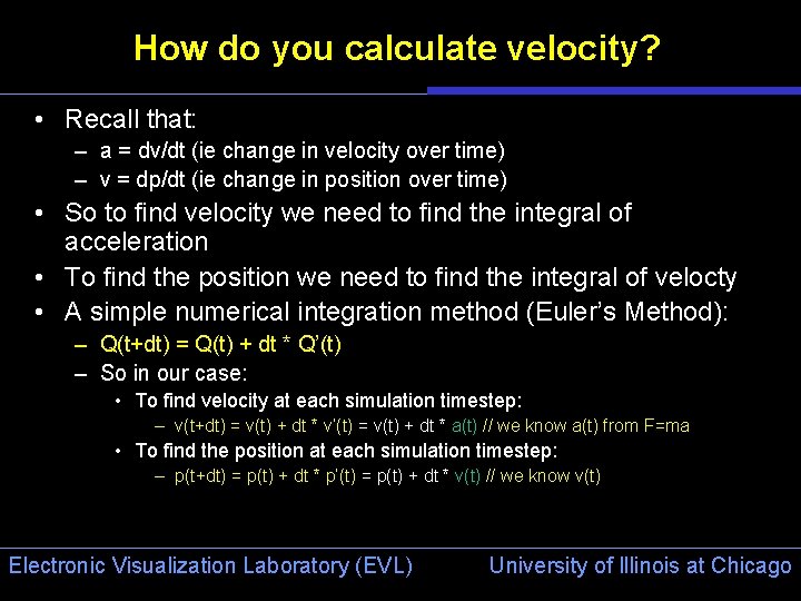
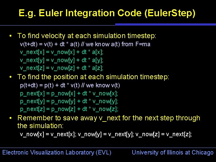
How do you calculate velocity? • Recall that: – a = dv/dt (ie change in velocity over time) – v = dp/dt (ie change in position over time) • So to find velocity we need to find the integral of acceleration • To find the position we need to find the integral of velocty • A simple numerical integration method (Euler’s Method): – Q(t+dt) = Q(t) + dt * Q’(t) – So in our case: • To find velocity at each simulation timestep: – v(t+dt) = v(t) + dt * v’(t) = v(t) + dt * a(t) // we know a(t) from F=ma • To find the position at each simulation timestep: – p(t+dt) = p(t) + dt * p’(t) = p(t) + dt * v(t) // we know v(t) Electronic Visualization Laboratory (EVL) University of Illinois at Chicago

E. g. Euler Integration Code (Euler. Step) • To find velocity at each simulation timestep: v(t+dt) = v(t) + dt * a(t) // we know a(t) from F=ma v_next[x] = v_now[x] + dt * a[x]; v_next[y] = v_now[y] + dt * a[y]; v_next[z] = v_now[z] + dt * a[z]; • To find the position at each simulation timestep: p(t+dt) = p(t) + dt * v(t) // we know v(t) p_next[x] = p_now[x] + dt * v_now[x]; p_next[y] = p_now[y] + dt * v_now[y]; p_next[z] = p_now[z] + dt * v_now[z]; • Remember to save away v_next for the next step through the simulation: v_now[x] = v_next[x]; v_now[y] = v_next[y]; v_now[z] = v_next[z]; Electronic Visualization Laboratory (EVL) University of Illinois at Chicago

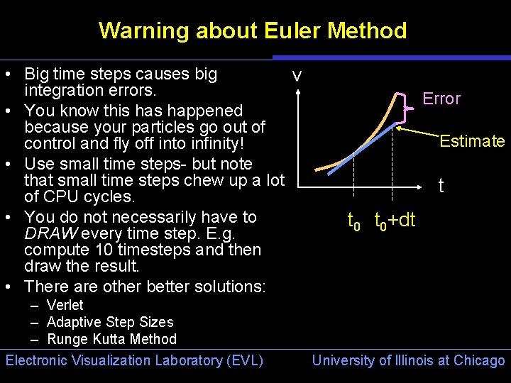
Warning about Euler Method • Big time steps causes big v integration errors. • You know this happened because your particles go out of control and fly off into infinity! • Use small time steps- but note that small time steps chew up a lot of CPU cycles. • You do not necessarily have to DRAW every time step. E. g. compute 10 timesteps and then draw the result. • There are other better solutions: – Verlet – Adaptive Step Sizes – Runge Kutta Method Electronic Visualization Laboratory (EVL) Error Estimate t t 0+dt University of Illinois at Chicago

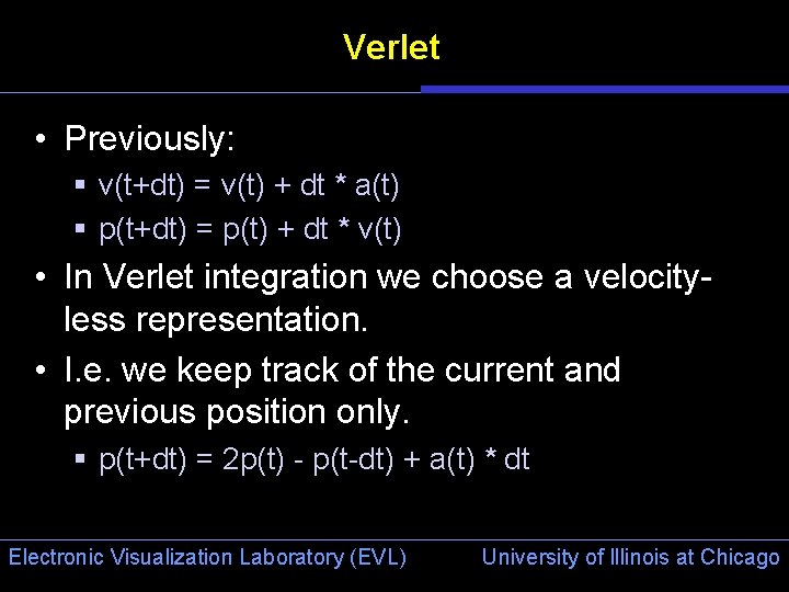
Verlet • Previously: § v(t+dt) = v(t) + dt * a(t) § p(t+dt) = p(t) + dt * v(t) • In Verlet integration we choose a velocityless representation. • I. e. we keep track of the current and previous position only. § p(t+dt) = 2 p(t) - p(t-dt) + a(t) * dt Electronic Visualization Laboratory (EVL) University of Illinois at Chicago

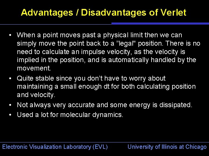
Advantages / Disadvantages of Verlet • When a point moves past a physical limit then we can simply move the point back to a ”legal" position. There is no need to calculate an impulse velocity, as the velocity is implied in the position, and is automatically handled by the movement. • Quite stable since you don’t have to worry about maintaining a small enough dt for both calculating position and velocity. • Not always very accurate and some energy is dissipated. • Used a lot for molecular dynamics. Electronic Visualization Laboratory (EVL) University of Illinois at Chicago

Computing Forces • Remember your particles are accelerating due to some Force that acts on it. • Gravity: – Easy: F = mg where g is the acceleration due to gravity: • a[x]=0; a[y]=9. 8 ms-2; a[z]=0; – Use this to compute F and add this to the force. Accumulator parameter. • Viscous Drag: – Like partcle moving thru water – F=-kd*V – Kd is coefficient of drag: basically it acts in the opposite direction of the Velocity of your particle. – Again apply the F by adding it to the force. Accumulator. • Damped Spring: – See next slide Electronic Visualization Laboratory (EVL) University of Illinois at Chicago

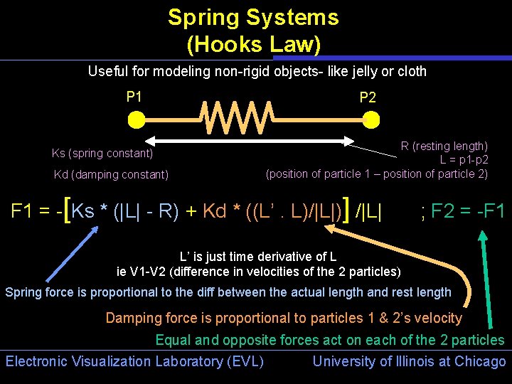
Spring Systems (Hooks Law) Useful for modeling non-rigid objects- like jelly or cloth P 1 P 2 Ks (spring constant) Kd (damping constant) R (resting length) L = p 1 -p 2 (position of particle 1 – position of particle 2) F 1 = -[Ks * (|L| - R) + Kd * ((L’. L)/|L|)] /|L| ; F 2 = -F 1 L’ is just time derivative of L ie V 1 -V 2 (difference in velocities of the 2 particles) Spring force is proportional to the diff between the actual length and rest length Damping force is proportional to particles 1 & 2’s velocity Equal and opposite forces act on each of the 2 particles Electronic Visualization Laboratory (EVL) University of Illinois at Chicago

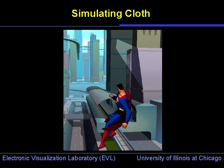
Simulating Cloth Electronic Visualization Laboratory (EVL) University of Illinois at Chicago

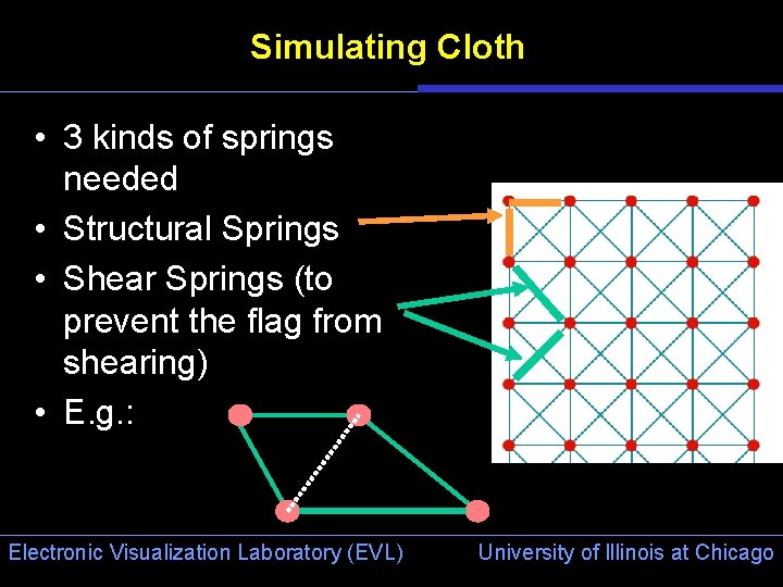
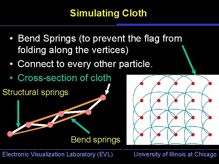
Simulating Cloth • 3 kinds of springs needed • Structural Springs • Shear Springs (to prevent the flag from shearing) • E. g. : Electronic Visualization Laboratory (EVL) University of Illinois at Chicago

Simulating Cloth • Bend Springs (to prevent the flag from folding along the vertices) • Connect to every other particle. • Cross-section of cloth Structural springs Bend springs Electronic Visualization Laboratory (EVL) University of Illinois at Chicago

Making Blobs • • • Gish 1 (www. chroniclogic. com/gish. htm) www. youtube. com/watch? v=5 Wz. GQQOIcp 8 Gish 2 Physics (128 particles) www. youtube. com/watch? v=TTcq. Zh. Qnr. Xw Bloft Soft Body Physics: bloft. hardwire. cz Electronic Visualization Laboratory (EVL) University of Illinois at Chicago

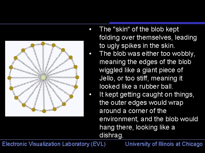
• • • The "skin" of the blob kept folding over themselves, leading to ugly spikes in the skin. The blob was either too wobbly, meaning the edges of the blob wiggled like a giant piece of Jello, or too stiff, meaning it looked like a rubber ball. It kept getting caught on things, the outer edges would wrap around a corner of the environment, and the blob would hang there, looking like a dishrag. Electronic Visualization Laboratory (EVL) University of Illinois at Chicago

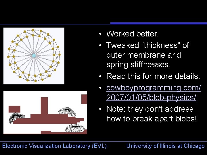
• Worked better. • Tweaked “thickness” of outer membrane and spring stiffnesses. • Read this for more details: • cowboyprogramming. com/ 2007/01/05/blob-physics/ • Note: they don’t address how to break apart blobs! Electronic Visualization Laboratory (EVL) University of Illinois at Chicago

Handling Collisions • Particles often bounce off surfaces. 1. Need to detect when a collision has occurred. 2. Need to determine the correct response to the collision. Electronic Visualization Laboratory (EVL) University of Illinois at Chicago

Detecting Collision • General Collision problem is complex: – Particle/Plane Collision – we will look at this one coz it’s easy way to start – Plane/Plane Collision – Edge/Plane Collision Electronic Visualization Laboratory (EVL) University of Illinois at Chicago

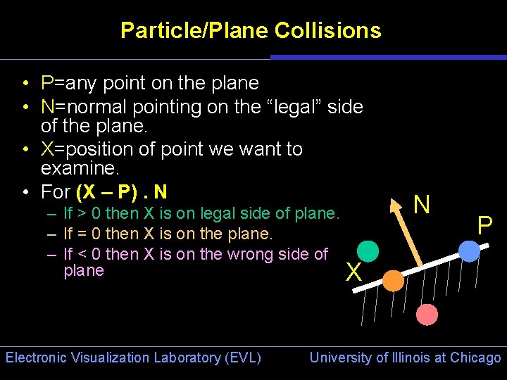
Particle/Plane Collisions • P=any point on the plane • N=normal pointing on the “legal” side of the plane. • X=position of point we want to examine. • For (X – P). N – If > 0 then X is on legal side of plane. – If = 0 then X is on the plane. – If < 0 then X is on the wrong side of plane X Electronic Visualization Laboratory (EVL) N P University of Illinois at Chicago

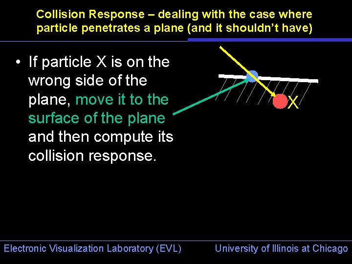
Collision Response – dealing with the case where particle penetrates a plane (and it shouldn’t have) • If particle X is on the wrong side of the plane, move it to the surface of the plane and then compute its collision response. Electronic Visualization Laboratory (EVL) X University of Illinois at Chicago

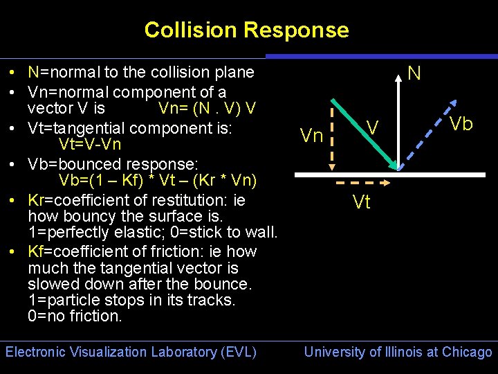
Collision Response • N=normal to the collision plane • Vn=normal component of a vector V is Vn= (N. V) V • Vt=tangential component is: Vt=V-Vn • Vb=bounced response: Vb=(1 – Kf) * Vt – (Kr * Vn) • Kr=coefficient of restitution: ie how bouncy the surface is. 1=perfectly elastic; 0=stick to wall. • Kf=coefficient of friction: ie how much the tangential vector is slowed down after the bounce. 1=particle stops in its tracks. 0=no friction. Electronic Visualization Laboratory (EVL) N Vn V Vb Vt University of Illinois at Chicago

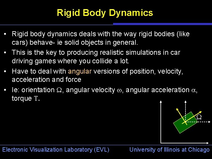
Rigid Body Dynamics • Rigid body dynamics deals with the way rigid bodies (like cars) behave- ie solid objects in general. • This is the key to producing realistic simulations in car driving games where you collide a lot. • Have to deal with angular versions of position, velocity, acceleration and force • Ie: orientation W, angular velocity w, angular acceleration a, torque T. W Electronic Visualization Laboratory (EVL) University of Illinois at Chicago

Rigid Body Dynamics • The gist is: – Calculate Center of Mass and Moment of Inertia at the Center of Mass – Moment of inertia is measure of the resistance of a body to angular acceleration: different for different shaped objects. Usually physics engine provide a # of preset shapes. – Center of Mass is the point where the entire mass of the object appears to reside. – Set body’s initial position, orientation, linear & angular velocities. – Figure out all forces acting on the body, including their points of application. (e. g. gravity & collision). – Sum all the forces and divide by total mass to find CM’s linear acceleration (ie F=ma). – Compute the total Torque at the CM. Torque is what causes angular acceleration (angular analog of Force). – Divide Torque by moment of inertia to find angular acceleration. – Numerically integrate linear and angular acceleration to get linear velocity, position, angular velocity, and orientation. – You deal with the entire body from its center of mass. – When rigid bodies collide you need to compute the point of intersection and determine how that collision causes change in angular as well as linear components. • • You will need to study the references in depth to figure out how to implement this. Would make a good Independent Study or MS project- if anyone is interested Electronic Visualization Laboratory (EVL) University of Illinois at Chicago

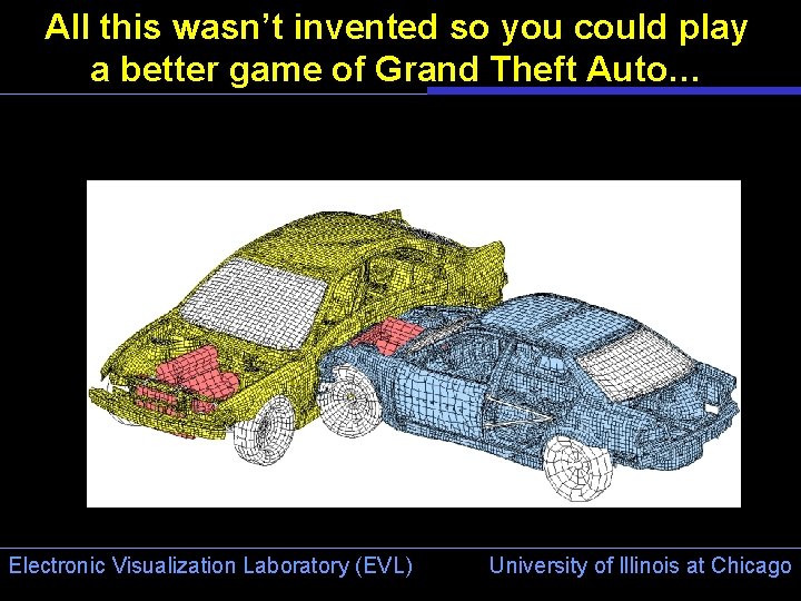
All this wasn’t invented so you could play a better game of Grand Theft Auto… Electronic Visualization Laboratory (EVL) University of Illinois at Chicago

Molecular Dynamics Folding Proteins Electronic Visualization Laboratory (EVL) University of Illinois at Chicago

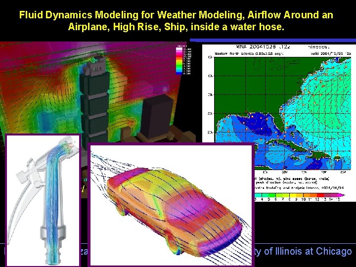
Fluid Dynamics Modeling for Weather Modeling, Airflow Around an Airplane, High Rise, Ship, inside a water hose. Electronic Visualization Laboratory (EVL) University of Illinois at Chicago

References “May the FORCE be with you. ” • Physics for Game Developers – David M. Bourg: O’Reilly & Associates. [highly recommended] Open Dynamics Engine: www. ode. org Tokamak Physics Engine: www. tokamakphysics. com SIGGRAPH Course Notes 34, 1995– www. siggraph. org Rigid Body Dynamics: Chris Hecker www. d 6. com/users/checker Jason’s Particle Systems C++ Class: www. evl. uic. edu/cavern/rg/20030201_leigh/ • Numerical Solvers: www. gamasutra. com/features/20000215/lander_01. htm • http: //www. evl. uic. edu/cavern/rg/20030201_leigh/diffyq. html • • • Electronic Visualization Laboratory (EVL) University of Illinois at Chicago

References • http: //en. wikipedia. org/wiki/Equations_of_motion • http: //www. gamasutra. com/resource_guide/20030121/jacobson_01. sht ml • http: //cowboyprogramming. com/2007/01/05/blob-physics/ • http: //www. gamasutra. com/view/feature/1549/practical_fluid_dynamics_ part_1. php • Verlet, L. "Computer experiments on classical fluids. I. Thermodynamical properties of Lennard-Jones molecules", Phys. Rev. , 159, 98 -103 (1967). • Witkin, Andrew and David Baraff, "Physically Based Modeling: Principles and Practice", Siggraph ’ 97 course notes, 1997. • http: //www. cs. cmu. edu/~baraff/sigcourse/index. html Electronic Visualization Laboratory (EVL) University of Illinois at Chicago

Adaptive Step Sizes • Ideally we want the step-size (dt) to be as big as possible so we can do as few calculations as possible. • But with bigger step sizes you incorporate more errors and your system can eventually destabilize. • So small step sizes are usually needed. Unfortunately smaller step sizes can take a long time. • You don’t want to force a small step size all the time if possible. Electronic Visualization Laboratory (EVL) University of Illinois at Chicago

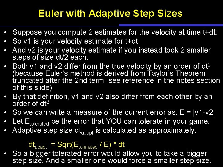
Euler with Adaptive Step Sizes • Suppose you compute 2 estimates for the velocity at time t+dt: • So v 1 is your velocity estimate for t+dt • And v 2 is your velocity estimate if you instead took 2 smaller steps of size dt/2 each. • Both v 1 and v 2 differ from the true velocity by an order of dt 2 (because Euler’s method is derived from Taylor’s Theorem truncated after the 2 nd term- see reference in the notes section of this slide) • By that definition, v 1 and v 2 also differ from each other by an order of dt 2 • So we can write a measure of the current error as: E = |v 1 -v 2| • Let Etolerated be the error that YOU can tolerate in your game. • Adaptive step size dtadapt is calculated as approximately: dtadapt = Sqrt(Etolerated / E) * dt • So a bigger tolerated error would allow. University you to take a bigger Electronic Visualization Laboratory (EVL) of Illinois at Chicago step size. And a smaller one would force a smaller step size.

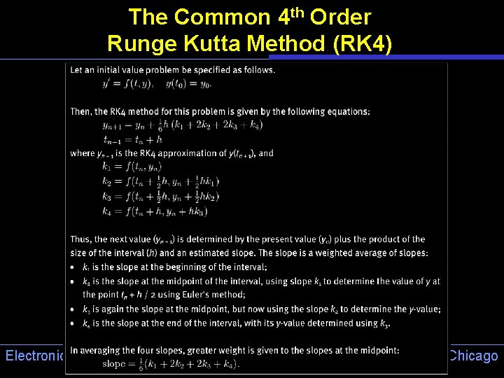
The Common 4 th Order Runge Kutta Method (RK 4) Electronic Visualization Laboratory (EVL) University of Illinois at Chicago

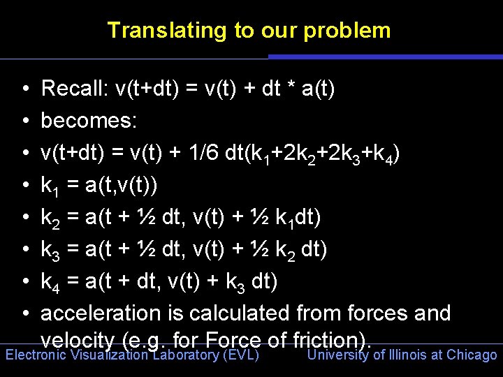
Translating to our problem • • Recall: v(t+dt) = v(t) + dt * a(t) becomes: v(t+dt) = v(t) + 1/6 dt(k 1+2 k 2+2 k 3+k 4) k 1 = a(t, v(t)) k 2 = a(t + ½ dt, v(t) + ½ k 1 dt) k 3 = a(t + ½ dt, v(t) + ½ k 2 dt) k 4 = a(t + dt, v(t) + k 3 dt) acceleration is calculated from forces and velocity (e. g. for Force of friction). Electronic Visualization Laboratory (EVL) University of Illinois at Chicago

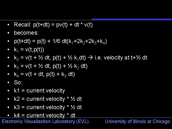
• • • Recall: p(t+dt) = pv(t) + dt * v(t) becomes: p(t+dt) = p(t) + 1/6 dt(k 1+2 k 2+2 k 3+k 4) k 1 = v(t, p(t)) k 2 = v(t + ½ dt, p(t) + ½ k 1 dt) i. e. velocity at t+½ dt k 3 = v(t + ½ dt, p(t) + ½ k 2 dt) k 4 = v(t + dt, p(t) + k 3 dt) So: k 1 = current velocity k 2 = current velocity * ½ dt k 3 = current velocity * ½ dt k 4 = current velocity * dt Electronic Visualization Laboratory (EVL) University of Illinois at Chicago