CS 412413 Introduction to Compilers Radu Rugina Lecture

CS 412/413 Introduction to Compilers Radu Rugina Lecture 21: More About Dataflow Analysis 13 Mar 02 CS 412/413 Spring 2002 Introduction to Compilers

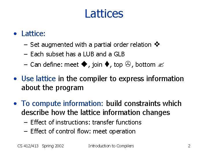
Lattices • Lattice: – Set augmented with a partial order relation – Each subset has a LUB and a GLB – Can define: meet , join , top , bottom • Use lattice in the compiler to express information about the program • To compute information: build constraints which describe how the lattice information changes – Effect of instructions: transfer functions – Effect of control flow: meet operation CS 412/413 Spring 2002 Introduction to Compilers 2

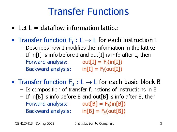
Transfer Functions • Let L = dataflow information lattice • Transfer function FI : L L for each instruction I – Describes how I modifies the information in the lattice – If in[I] is info before I and out[I] is info after I, then Forward analysis: out[I] = FI(in[I]) Backward analysis: in[I] = FI(out[I]) • Transfer function FB : L L for each basic block B – Is composition of transfer functions of instructions in B – If in[B] is info before B and out[B] is info after B, then Forward analysis: out[B] = FB(in[B]) Backward analysis: in[B] = FB(out[B]) CS 412/413 Spring 2002 Introduction to Compilers 3

Monotonicity and Distributivity • Two important properties of transfer functions • Monotonicity: function F : L L is monotonic if x y implies F(x) F(y) • Distributivity: function F : L L is distributive if F(x y) = F(x) F(y) • Property: F is monotonic iff F(x y) F(x) F(y) - any distributive function is monotonic! CS 412/413 Spring 2002 Introduction to Compilers 4

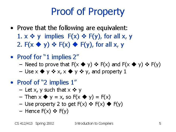
Proof of Property • Prove that the following are equivalent: 1. x y implies F(x) F(y), for all x, y 2. F(x y) F(x) F(y), for all x, y • Proof for “ 1 implies 2” – Need to prove that F(x y) F(x) and F(x y) F(y) – Use x y x, x y y, and property 1 • Proof of “ 2 implies 1” – – Let x, y such that x y Then x y = x, so F(x y) = F(x) Use property 2 to get F(x) F(y) Hence F(x) F(y) CS 412/413 Spring 2002 Introduction to Compilers 5

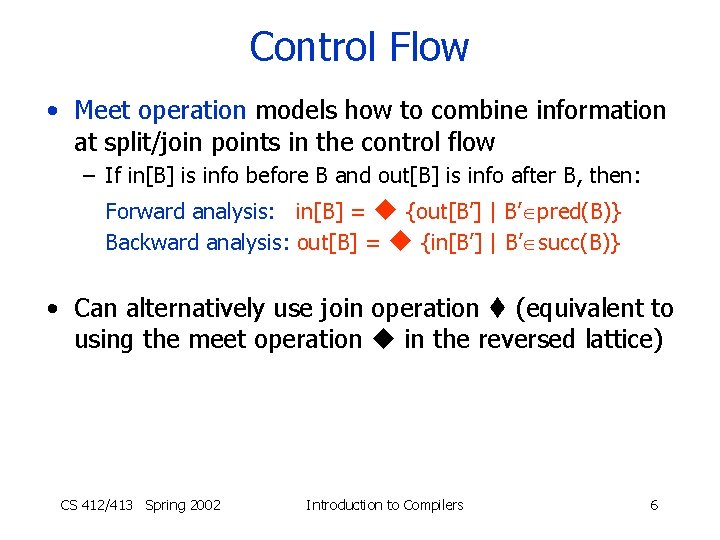
Control Flow • Meet operation models how to combine information at split/join points in the control flow – If in[B] is info before B and out[B] is info after B, then: Forward analysis: in[B] = {out[B’] | B’ pred(B)} Backward analysis: out[B] = {in[B’] | B’ succ(B)} • Can alternatively use join operation (equivalent to using the meet operation in the reversed lattice) CS 412/413 Spring 2002 Introduction to Compilers 6

Monotonicity of Meet • Meet operation is also monotonic over L x L: x 1 y 1 and x 2 y 2 implies (x 1 x 2) (y 1 y 2) • Proof: – any lower bound of {x 1, x 2} is also a lower bound of {y 1, y 2}, because x 1 y 1 and x 2 y 2 – x 1 x 2 is a lower bound of {x 1, x 2} – So x 1 x 2 is a lower bound of {y 1, y 2} – But y 1 y 2 is the greatest lower bound of {y 1, y 2} – Hence (x 1 x 2) (y 1 y 2) CS 412/413 Spring 2002 Introduction to Compilers 7

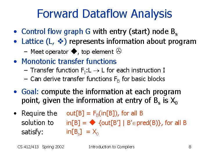
Forward Dataflow Analysis • Control flow graph G with entry (start) node Bs • Lattice (L, ) represents information about program – Meet operator , top element • Monotonic transfer functions – Transfer function FI: L L for each instruction I – Can derive transfer functions FB for basic blocks • Goal: compute the information at each program point, given the information at entry of Bs is X 0 • Require the solution to satisfy: CS 412/413 Spring 2002 out[B] = FB(in[B]), for all B in[B] = {out[B’] | B’ pred(B)}, for all B in[Bs] = X 0 Introduction to Compilers 8

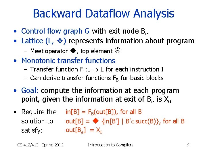
Backward Dataflow Analysis • Control flow graph G with exit node Be • Lattice (L, ) represents information about program – Meet operator , top element • Monotonic transfer functions – Transfer function FI: L L for each instruction I – Can derive transfer functions FB for basic blocks • Goal: compute the information at each program point, given the information at exit of Be is X 0 • Require the solution to satisfy: CS 412/413 Spring 2002 in[B] = FB(out[B]), for all B out[B] = {in[B’] | B’ succ(B)}, for all B out[Be] = X 0 Introduction to Compilers 9

Dataflow Equations • The constraints are called dataflow equations: out[B] = FB(in[B]), for all B in[B] = {out[B’] | B’ pred(B)}, for all B in[Bs] = X 0 • Solve equations: use an iterative algorithm – Initialize in[Bs] = X 0 – Initialize everything else to – Repeatedly apply rules – Stop when reach a fixed point CS 412/413 Spring 2002 Introduction to Compilers 10

Algorithm in[BS] = X 0 out[B] = , for all B Repeat For each basic block B Bs in[B] = {out[B’] | B’ pred(B)} For each basic block B out[B] = FB(in[B]) Until no change CS 412/413 Spring 2002 Introduction to Compilers 11

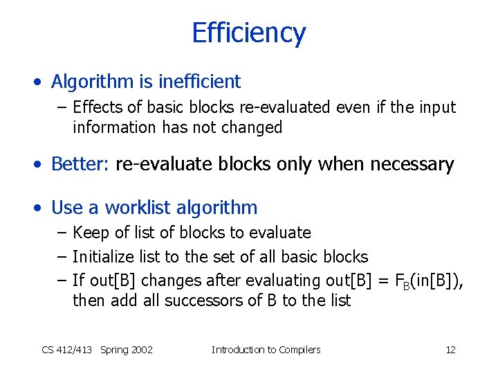
Efficiency • Algorithm is inefficient – Effects of basic blocks re-evaluated even if the input information has not changed • Better: re-evaluate blocks only when necessary • Use a worklist algorithm – Keep of list of blocks to evaluate – Initialize list to the set of all basic blocks – If out[B] changes after evaluating out[B] = FB(in[B]), then add all successors of B to the list CS 412/413 Spring 2002 Introduction to Compilers 12

Worklist Algorithm in[BS] = X 0 out[B] = , for all B worklist = set of all basic blocks B Repeat Remove a node B from the worklist in[B] = {out[B’] | B’ pred(B)} out[B] = FB(in[B]) if out[B] has changed, then worklist = worklist succ(B) Until worklist = CS 412/413 Spring 2002 Introduction to Compilers 13

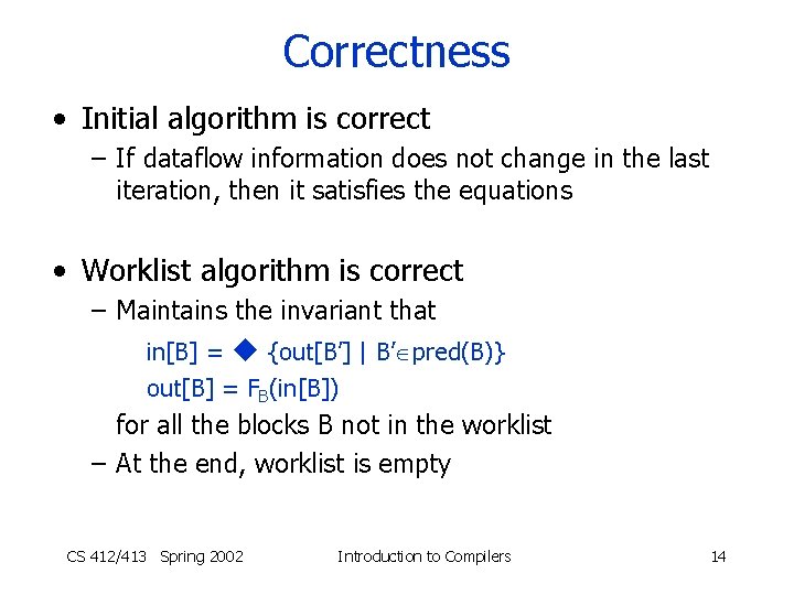
Correctness • Initial algorithm is correct – If dataflow information does not change in the last iteration, then it satisfies the equations • Worklist algorithm is correct – Maintains the invariant that in[B] = {out[B’] | B’ pred(B)} out[B] = FB(in[B]) for all the blocks B not in the worklist – At the end, worklist is empty CS 412/413 Spring 2002 Introduction to Compilers 14

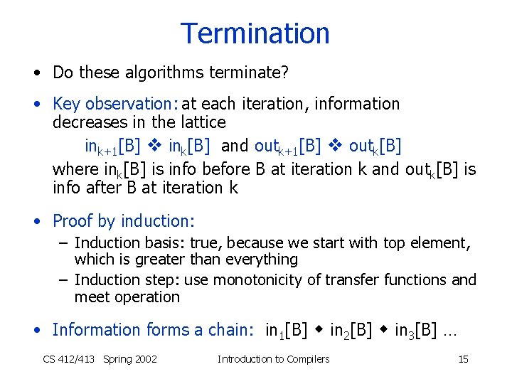
Termination • Do these algorithms terminate? • Key observation: at each iteration, information decreases in the lattice ink+1[B] ink[B] and outk+1[B] outk[B] where ink[B] is info before B at iteration k and outk[B] is info after B at iteration k • Proof by induction: – Induction basis: true, because we start with top element, which is greater than everything – Induction step: use monotonicity of transfer functions and meet operation • Information forms a chain: in 1[B] in 2[B] in 3[B] … CS 412/413 Spring 2002 Introduction to Compilers 15

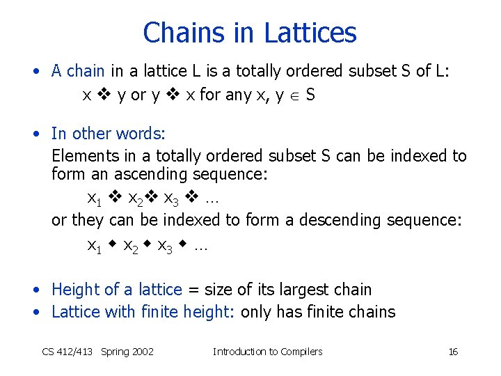
Chains in Lattices • A chain in a lattice L is a totally ordered subset S of L: x y or y x for any x, y S • In other words: Elements in a totally ordered subset S can be indexed to form an ascending sequence: x 1 x 2 x 3 … or they can be indexed to form a descending sequence: x 1 x 2 x 3 … • Height of a lattice = size of its largest chain • Lattice with finite height: only has finite chains CS 412/413 Spring 2002 Introduction to Compilers 16

Termination • In the iterative algorithm, for each block B: {in 1[B], in 2[B], …} is a chain in the lattice, because transfer functions and meet operation are monotonic • If lattice has finite height then these sets are finite, i. e. there is a number k such that ini[B] = ini+1[B], for all i k and all B • If ini[B] = ini+1[B] then also outi[B] = outi+1[B] • Hence algorithm terminates in at most k iterations • To summarize: dataflow analysis terminates if 1. Transfer functions are monotonic 2. Lattice has finite height CS 412/413 Spring 2002 Introduction to Compilers 17

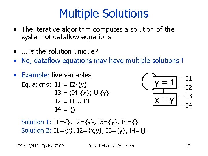
Multiple Solutions • The iterative algorithm computes a solution of the system of dataflow equations • … is the solution unique? • No, dataflow equations may have multiple solutions ! • Example: live variables Equations: I 1 I 3 I 2 I 4 = = I 2 -{y} (I 4 -{x}) U {y} I 1 U I 3 {} y=1 x=y I 1 I 2 I 3 I 4 Solution 1: I 1={}, I 2={y}, I 3={y}, I 4={} Solution 2: I 1={x}, I 2={x, y}, I 3={y}, I 4={} CS 412/413 Spring 2002 Introduction to Compilers 18

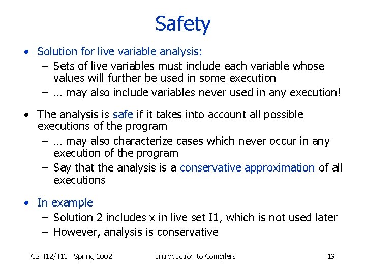
Safety • Solution for live variable analysis: – Sets of live variables must include each variable whose values will further be used in some execution – … may also include variables never used in any execution! • The analysis is safe if it takes into account all possible executions of the program – … may also characterize cases which never occur in any execution of the program – Say that the analysis is a conservative approximation of all executions • In example – Solution 2 includes x in live set I 1, which is not used later – However, analysis is conservative CS 412/413 Spring 2002 Introduction to Compilers 19

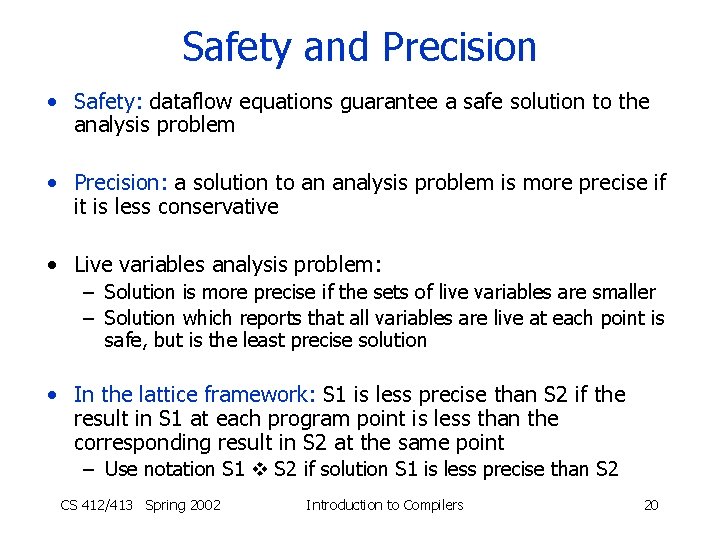
Safety and Precision • Safety: dataflow equations guarantee a safe solution to the analysis problem • Precision: a solution to an analysis problem is more precise if it is less conservative • Live variables analysis problem: – Solution is more precise if the sets of live variables are smaller – Solution which reports that all variables are live at each point is safe, but is the least precise solution • In the lattice framework: S 1 is less precise than S 2 if the result in S 1 at each program point is less than the corresponding result in S 2 at the same point – Use notation S 1 S 2 if solution S 1 is less precise than S 2 CS 412/413 Spring 2002 Introduction to Compilers 20

Maximal Fixed Point Solution • Property: among all the solutions to the system of dataflow equations, the iterative solution is the most precise • Intuition: – We start with the top element at each program point (i. e. most precise information) – Then refine the information at each iteration to satisfy the dataflow equations – Final result will be the closest to the top • Iterative solution for dataflow equations is called Maximal Fixed Point solution (MFP) • For any solution FP of the dataflow equations: FP CS 412/413 Spring 2002 Introduction to Compilers MFP 21

Meet Over Paths Solution • Is MFP the best solution to the analysis problem? • Another approach: consider a lattice framework, but use a different way to compute the solution – Let G be the control flow graph with start block B 0 – For each path pn=[B 0, B 1, …, Bn] from entry to block Bn: in[pn] = FBn-1 ( … (FB 1(FB 0(X 0)))) – Compute solution as in[Bn] = { in[pn] | all paths pn from B 0 to Bn} • This solution is the Meet Over Paths solution (MOP) CS 412/413 Spring 2002 Introduction to Compilers 22

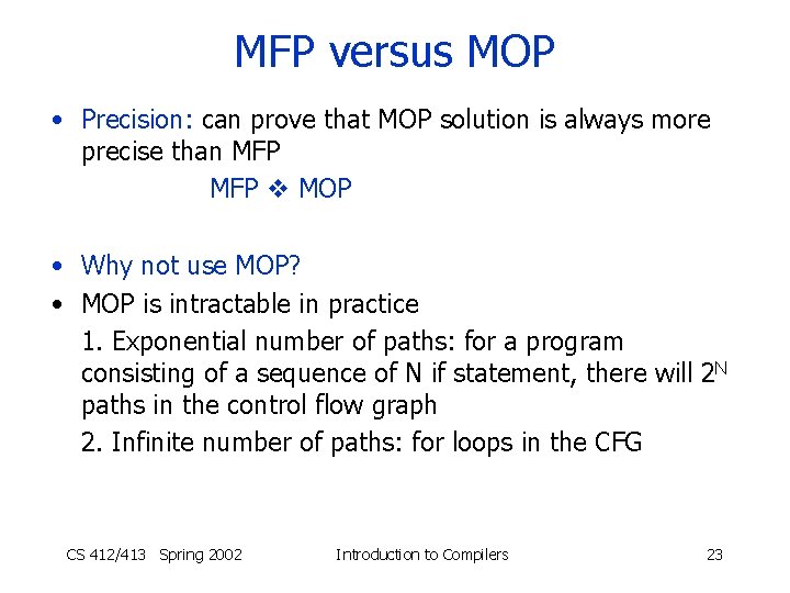
MFP versus MOP • Precision: can prove that MOP solution is always more precise than MFP MOP • Why not use MOP? • MOP is intractable in practice 1. Exponential number of paths: for a program consisting of a sequence of N if statement, there will 2 N paths in the control flow graph 2. Infinite number of paths: for loops in the CFG CS 412/413 Spring 2002 Introduction to Compilers 23

Importance of Distributivity • Property: if transfer functions are distributive, then the solution to the dataflow equations is identical to the meet-over-paths solution MFP = MOP • For distributive transfer functions, can compute the intractable MOP solution using the iterative fixedpoint algorithm CS 412/413 Spring 2002 Introduction to Compilers 24

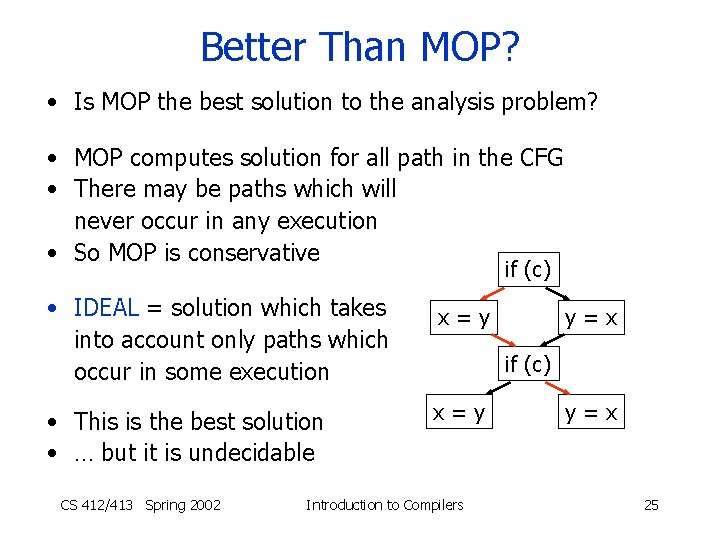
Better Than MOP? • Is MOP the best solution to the analysis problem? • MOP computes solution for all path in the CFG • There may be paths which will never occur in any execution • So MOP is conservative if (c) • IDEAL = solution which takes into account only paths which occur in some execution • This is the best solution • … but it is undecidable CS 412/413 Spring 2002 x=y y=x if (c) x=y Introduction to Compilers y=x 25

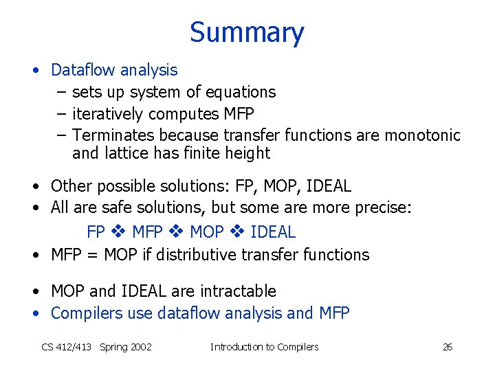
Summary • Dataflow analysis – sets up system of equations – iteratively computes MFP – Terminates because transfer functions are monotonic and lattice has finite height • Other possible solutions: FP, MOP, IDEAL • All are safe solutions, but some are more precise: FP MOP IDEAL • MFP = MOP if distributive transfer functions • MOP and IDEAL are intractable • Compilers use dataflow analysis and MFP CS 412/413 Spring 2002 Introduction to Compilers 26