CS 395 Adv Computer Graphics Introduction to ImageSpace
- Slides: 36

CS 395: Adv. Computer Graphics Introduction to Image-Space Methods Watt & Watt: Chapter 14 + readings Jack Tumblin jet@cs. northwestern. edu

Image Space Methods • A ‘Digital Image’ = a data structure for displayed images • ? What can it do, besides display? what can we change? – Position; offset, stretch, squeeze, smear, cut, … Try It! (Java Applets) http: //www. mrl. nyu. edu/~hertzman/nudge/ – Combine: Add, Subtract/ Overlay / Compositing – Separate: matte or ‘segmenting’ – Elaborate: make ‘more of the same’ picture

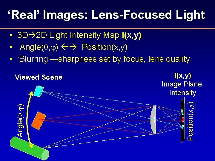
‘Real’ Images: Lens-Focused Light 3 D 2 D Light Intensity Map I(x, y) Angle( , ) Position(x, y) ‘Blurring’—sharpness set by focus, lens quality I(x, y) Image Plane Intensity Position(x, y) Viewed Scene Angle( , ) • • •

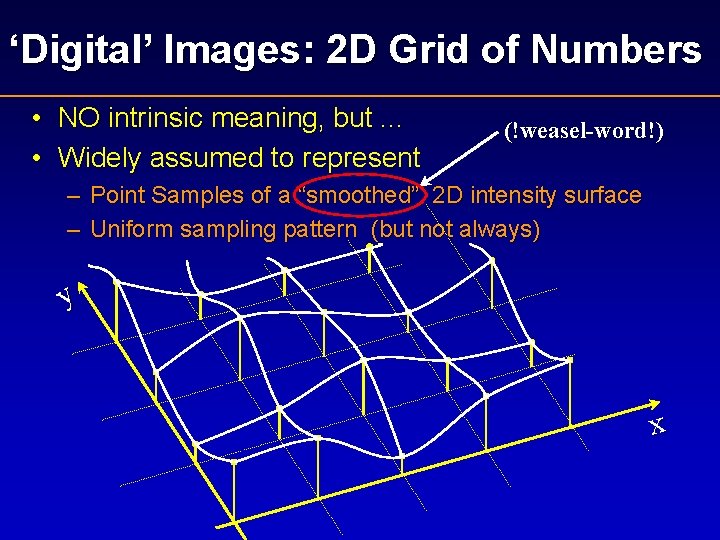
‘Digital’ Images: 2 D Grid of Numbers • NO intrinsic meaning, but. . . • Widely assumed to represent (!weasel-word!) – Point Samples of a “smoothed” 2 D intensity surface – Uniform sampling pattern (but not always) y x

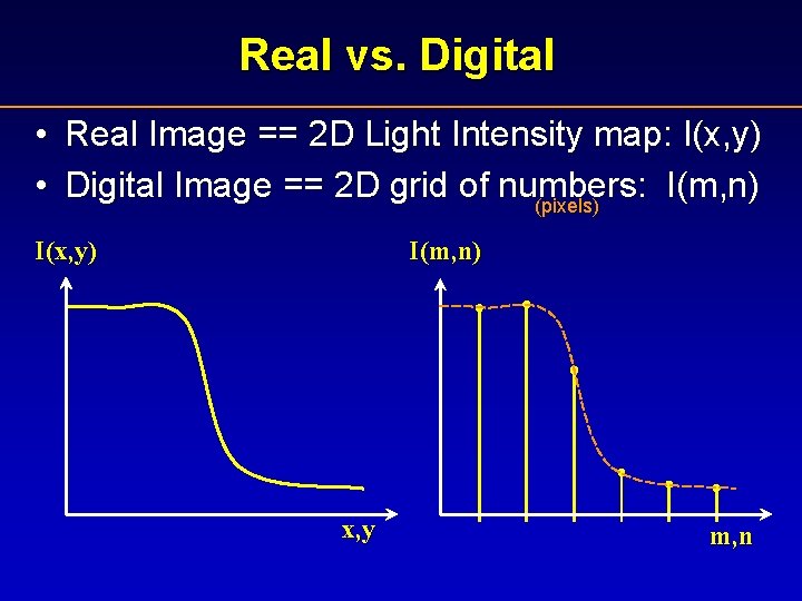
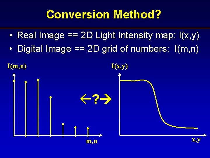
Real vs. Digital • Real Image == 2 D Light Intensity map: I(x, y) • Digital Image == 2 D grid of numbers: I(m, n) (pixels) I(x, y) I(m, n) x, y m, n

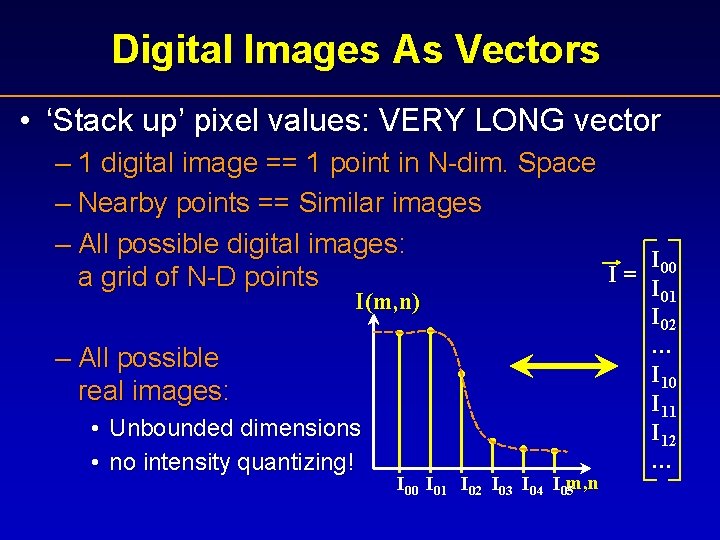
Digital Images As Vectors • ‘Stack up’ pixel values: VERY LONG vector – 1 digital image == 1 point in N-dim. Space – Nearby points == Similar images – All possible digital images: I 00 I= a grid of N-D points I 01 I(m, n) – All possible real images: • Unbounded dimensions • no intensity quantizing! I 00 I 01 I 02 I 03 I 04 I 05 m, n 01 I 02 … I 10 I 11 I 12 …

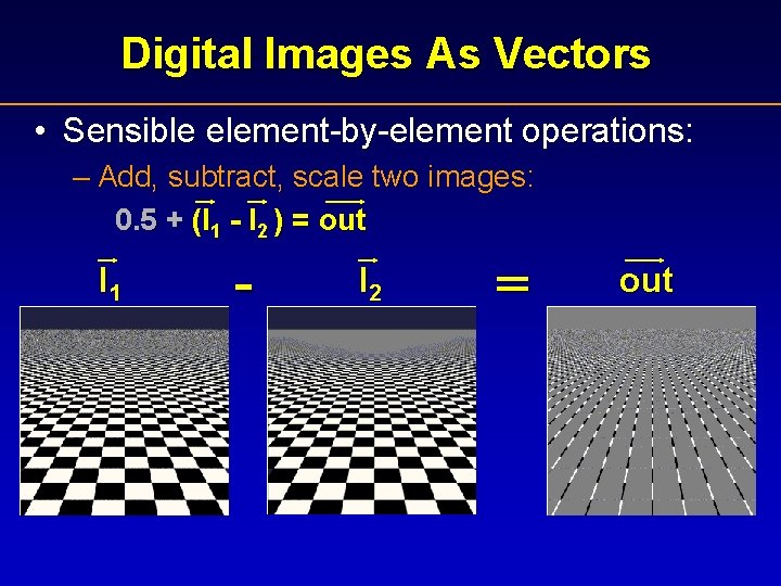
Digital Images As Vectors • Sensible element-by-element operations: – Add, subtract, scale two images: 0. 5 + (I 1 - I 2 ) = out I 1 - I 2 = out

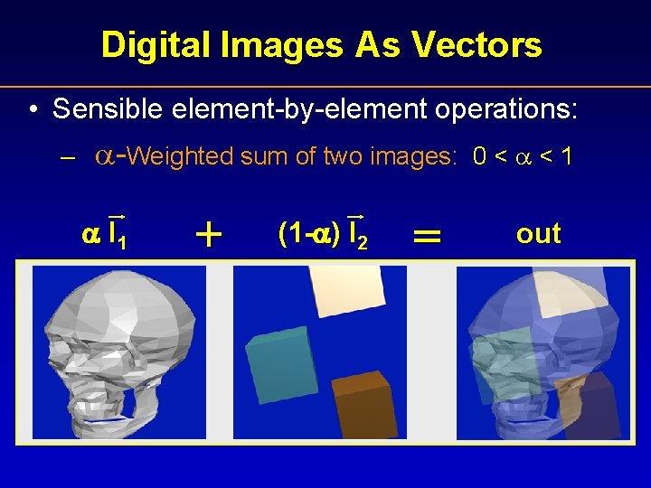
Digital Images As Vectors • Sensible element-by-element operations: – -Weighted sum of two images: I 1 + (1 - ) I 2 = 0< <1 out

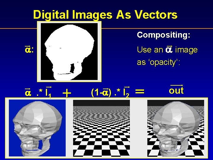
Digital Images As Vectors Compositing: Use an image as ‘opacity’: : . * I 1 + (1 - ). * I 2 = out

! NOT EQUIVALENT ! ? Digital image: pixel-by-pixel operations ? ? Real Image: point-by-point operations ? Source of much frustration & error! Digital Image == Real Image Also see Alvy Ray Smith’s article entitled: “A pixel is NOT a little square, a pixel is NOT a little square!” found here.

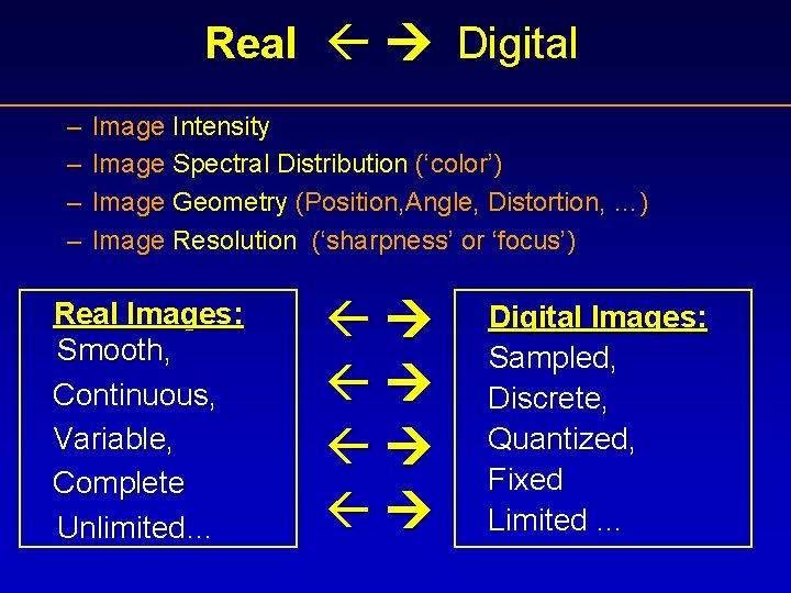
Real Digital – – Image Intensity Image Spectral Distribution (‘color’) Image Geometry (Position, Angle, Distortion, …) Image Resolution (‘sharpness’ or ‘focus’) Real Images: Smooth, Continuous, Variable, Complete Unlimited… Digital Images: Sampled, Discrete, Quantized, Fixed Limited …

Conversion Method? • Real Image == 2 D Light Intensity map: I(x, y) • Digital Image == 2 D grid of numbers: I(m, n) I(x, y) ? m, n x, y

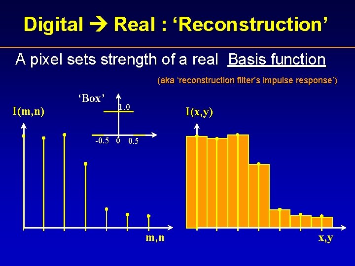
Digital Real : ‘Reconstruction’ A pixel sets strength of a real Basis function (aka ‘reconstruction filter’s impulse response’) I(m, n) ‘Box’ 1. 0 I(x, y) -0. 5 0 0. 5 m, n x, y

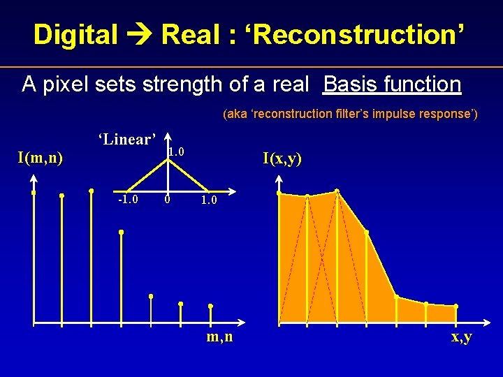
Digital Real : ‘Reconstruction’ A pixel sets strength of a real Basis function (aka ‘reconstruction filter’s impulse response’) I(m, n) ‘Linear’ -1. 0 0 I(x, y) 1. 0 m, n x, y

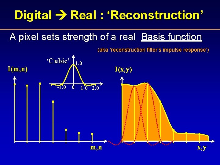
Digital Real : ‘Reconstruction’ A pixel sets strength of a real Basis function (aka ‘reconstruction filter’s impulse response’) I(m, n) ‘Cubic’ -1. 0 0 I(x, y) 1. 0 2. 0 m, n x, y

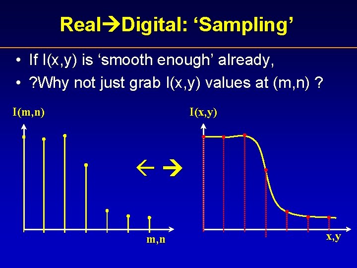
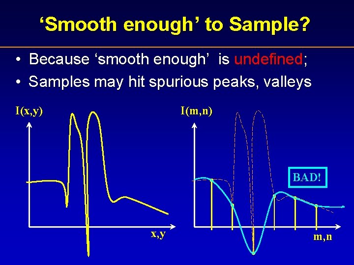
Real Digital: ‘Sampling’ • If I(x, y) is ‘smooth enough’ already, • ? Why not just grab I(x, y) values at (m, n) ? I(m, n) I(x, y) m, n x, y

‘Smooth enough’ to Sample? • Because ‘smooth enough’ is undefined; • Samples may hit spurious peaks, valleys I(x, y) I(m, n) BAD! x, y m, n

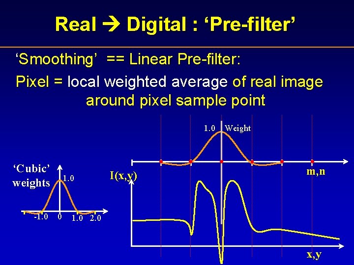
Real Digital : ‘Pre-filter’ ‘Smoothing’ == Linear Pre-filter: Pixel = local weighted average of real image around pixel sample point 1. 0 ‘Cubic’ weights -1. 0 0 I(x, y) Weight m, n 1. 0 2. 0 x, y

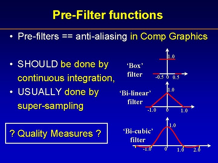
Pre-Filter functions • Pre-filters == anti-aliasing in Comp Graphics • SHOULD be done by continuous integration, • USUALLY done by super-sampling ? Quality Measures ? 1. 0 ‘Box’ filter -0. 5 0 0. 5 1. 0 ‘Bi-linear’ filter -1. 0 0 1. 0 ‘Bi-cubic’ filter -1. 0 0 1. 0 2. 0

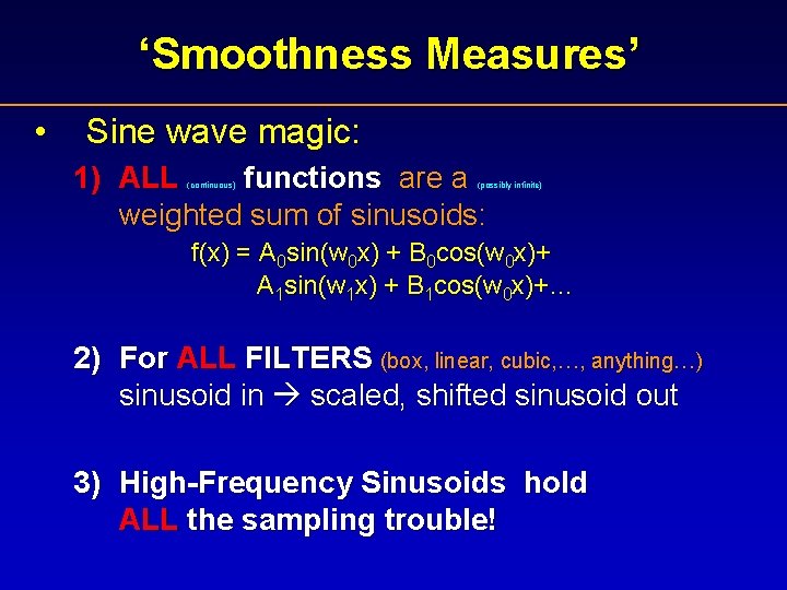
‘Smoothness Measures’ • Sine wave magic: 1) ALL functions are a weighted sum of sinusoids: (continuous) (possibly infinite) f(x) = A 0 sin(w 0 x) + B 0 cos(w 0 x)+ A 1 sin(w 1 x) + B 1 cos(w 0 x)+… 2) For ALL FILTERS (box, linear, cubic, …, anything…) sinusoid in scaled, shifted sinusoid out 3) High-Frequency Sinusoids hold ALL the sampling trouble!

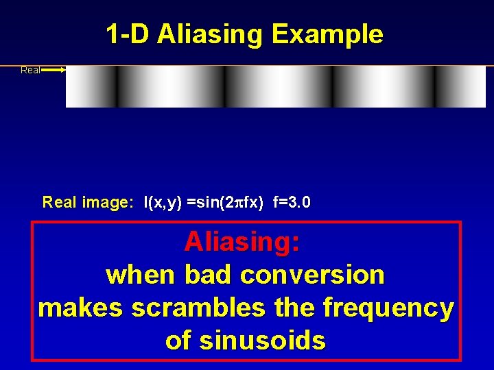
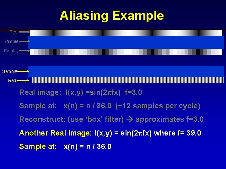
1 -D Aliasing Example Real image: I(x, y) =sin(2 fx) f=3. 0 Aliasing: when bad conversion makes scrambles the frequency of sinusoids

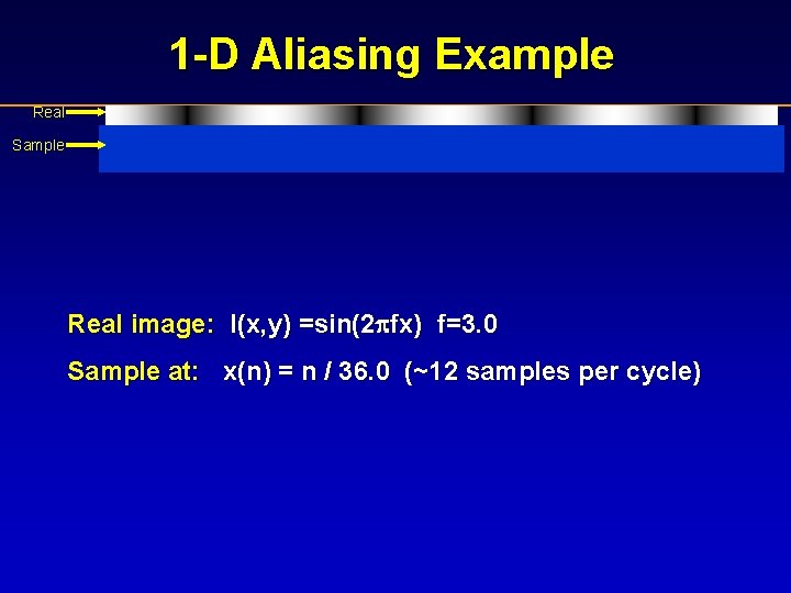
1 -D Aliasing Example Real Sample Real image: I(x, y) =sin(2 fx) f=3. 0 Sample at: x(n) = n / 36. 0 (~12 samples per cycle)

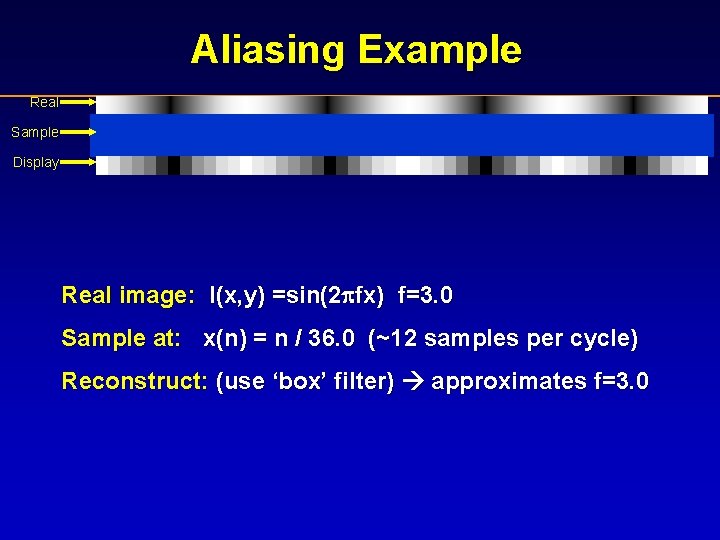
Aliasing Example Real Sample Display Real image: I(x, y) =sin(2 fx) f=3. 0 Sample at: x(n) = n / 36. 0 (~12 samples per cycle) Reconstruct: (use ‘box’ filter) approximates f=3. 0

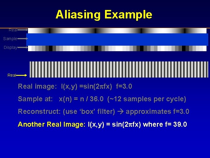
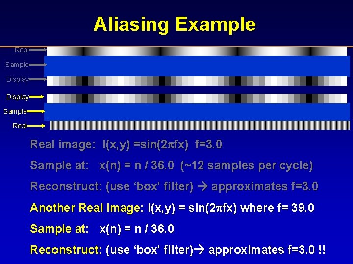
Aliasing Example Real Sample Display Real image: I(x, y) =sin(2 fx) f=3. 0 Sample at: x(n) = n / 36. 0 (~12 samples per cycle) Reconstruct: (use ‘box’ filter) approximates f=3. 0 Another Real Image: I(x, y) = sin(2 fx) where f= 39. 0

Aliasing Example Real Sample Display Sample Real image: I(x, y) =sin(2 fx) f=3. 0 Sample at: x(n) = n / 36. 0 (~12 samples per cycle) Reconstruct: (use ‘box’ filter) approximates f=3. 0 Another Real Image: I(x, y) = sin(2 fx) where f= 39. 0 Sample at: x(n) = n / 36. 0

Aliasing Example Real Sample Display Sample Real image: I(x, y) =sin(2 fx) f=3. 0 Sample at: x(n) = n / 36. 0 (~12 samples per cycle) Reconstruct: (use ‘box’ filter) approximates f=3. 0 Another Real Image: I(x, y) = sin(2 fx) where f= 39. 0 Sample at: x(n) = n / 36. 0 Reconstruct: (use ‘box’ filter) approximates f=3. 0 !!

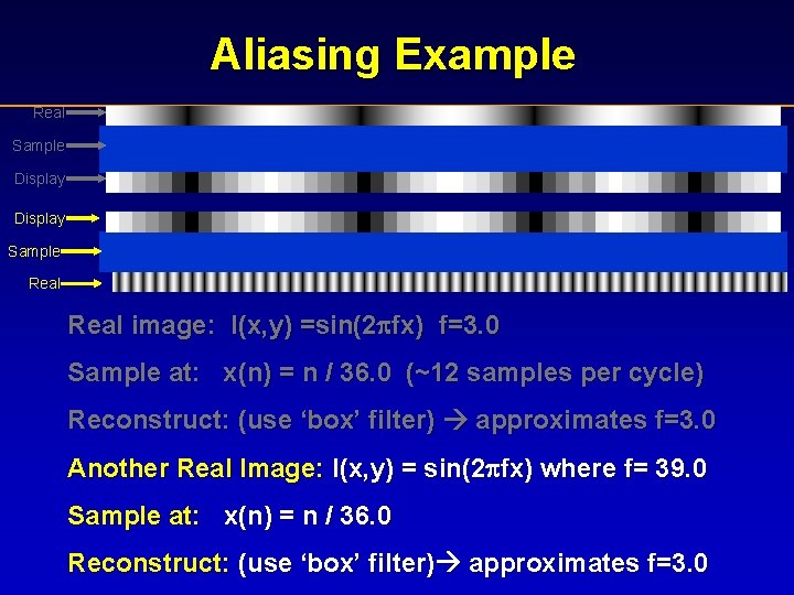
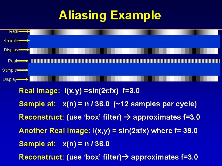
Aliasing Example Real Sample Display Sample Real image: I(x, y) =sin(2 fx) f=3. 0 Sample at: x(n) = n / 36. 0 (~12 samples per cycle) Reconstruct: (use ‘box’ filter) approximates f=3. 0 Another Real Image: I(x, y) = sin(2 fx) where f= 39. 0 Sample at: x(n) = n / 36. 0 Reconstruct: (use ‘box’ filter) approximates f=3. 0

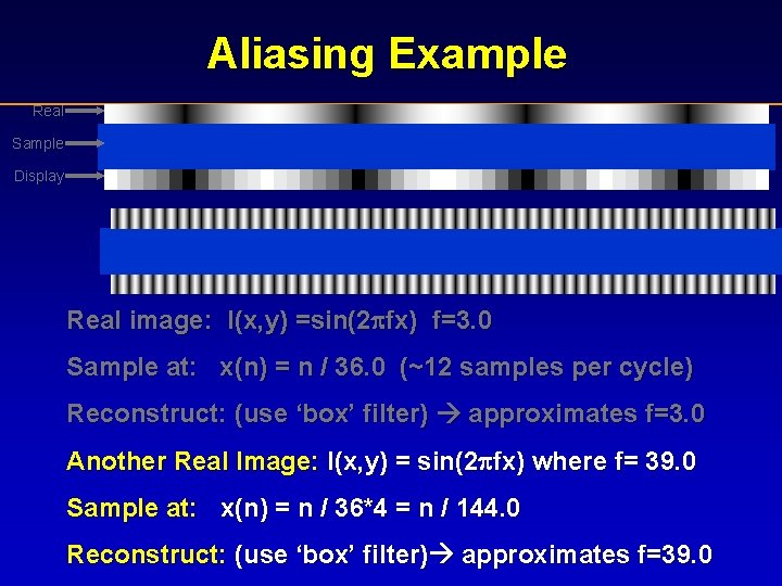
Aliasing Example Real Sample Display Real image: I(x, y) =sin(2 fx) f=3. 0 Sample at: x(n) = n / 36. 0 (~12 samples per cycle) Reconstruct: (use ‘box’ filter) approximates f=3. 0 Another Real Image: I(x, y) = sin(2 fx) where f= 39. 0 Sample at: x(n) = n / 36*4 = n / 144. 0 Reconstruct: (use ‘box’ filter) approximates f=39. 0

Conclusion: • Image-space manipulations must explicitly address real-digital (discrete-continuous) conversions to avoid aliasing artifacts. • Digital images are compact, indirect, ambiguous descriptions of light distributions

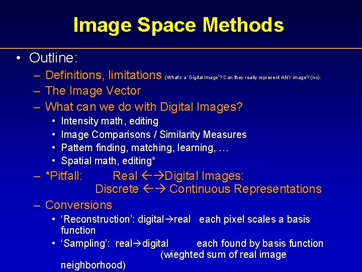
Image Space Methods • Outline: – – – Definitions, limitations (What’s a ‘Digital Image’? Can they really represent ANY image? (no). The Image Vector What can we do with Digital Images? • • Intensity math, editing Image Comparisons / Similarity Measures Pattern finding, matching, learning, … Spatial math, editing* – *Pitfall: Real Digital Images: Discrete Continuous Representations – Conversions • ‘Reconstruction’: digital real each pixel scales a basis function • ‘Sampling’: real digital each found by basis function (wieghted sum of real image neighborhood)

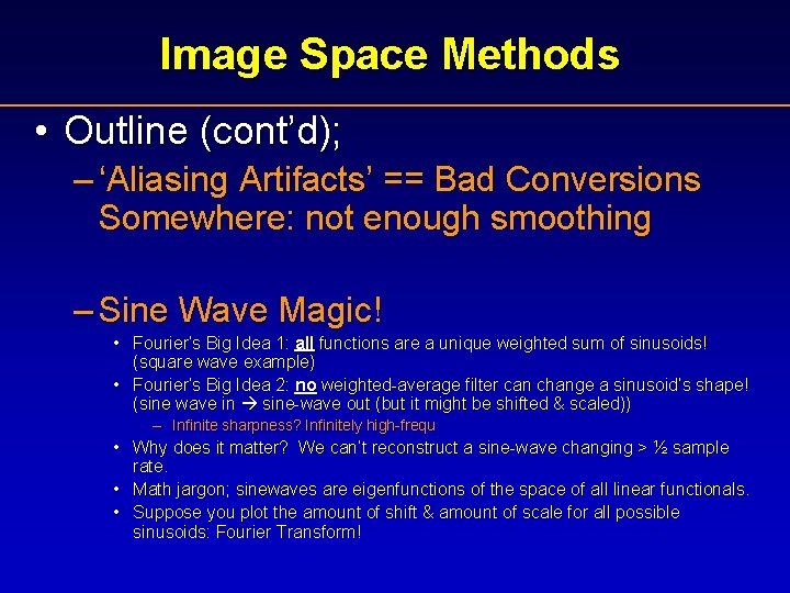
Image Space Methods • Outline (cont’d); – ‘Aliasing Artifacts’ == Bad Conversions Somewhere: not enough smoothing – Sine Wave Magic! • Fourier’s Big Idea 1: all functions are a unique weighted sum of sinusoids! (square wave example) • Fourier’s Big Idea 2: no weighted-average filter can change a sinusoid’s shape! (sine wave in sine-wave out (but it might be shifted & scaled)) – Infinite sharpness? Infinitely high-frequ • Why does it matter? We can’t reconstruct a sine-wave changing > ½ sample rate. • Math jargon; sinewaves are eigenfunctions of the space of all linear functionals. • Suppose you plot the amount of shift & amount of scale for all possible sinusoids: Fourier Transform!

Aliasing Example Real Sample Display Real image: I(x, y) =sin(2 fx) f=3. 0 Sample at: x(n) = n / 36. 0 (~12 samples per cycle) Reconstruct: (use ‘box’ filter) approximates f=3. 0 Another Real Image: I(x, y) = sin(2 fx) where f= 39. 0 Sample at: x(n) = n / 36. 0 Reconstruct: (use ‘box’ filter) approximates f=3. 0

SAFETY COPY

Reconstruction: Digital Real How to ‘Read Between the Pixels’

Pre-Filter: Real Digital

Image Space Methods • Intro: What can we do with images? • Re-sampling: Continuous & Discrete Filters – – Interpolation: What’s ‘in-between’ a pixel? Antialiasing: What makes a good sampling? Math Rigor: the Fourier Transform Examples: box, triangle, Mitchell-Netravali • Compositing: Transparency • Un-Compositing: Matte Separations • Further extensions: – – – Environment Matte Polynomial Texture Map Texture Elaboration, Image Inpainting(Sigg 2000)