CS 391 L Machine Learning Clustering Raymond J

CS 391 L: Machine Learning Clustering Raymond J. Mooney University of Texas at Austin 1

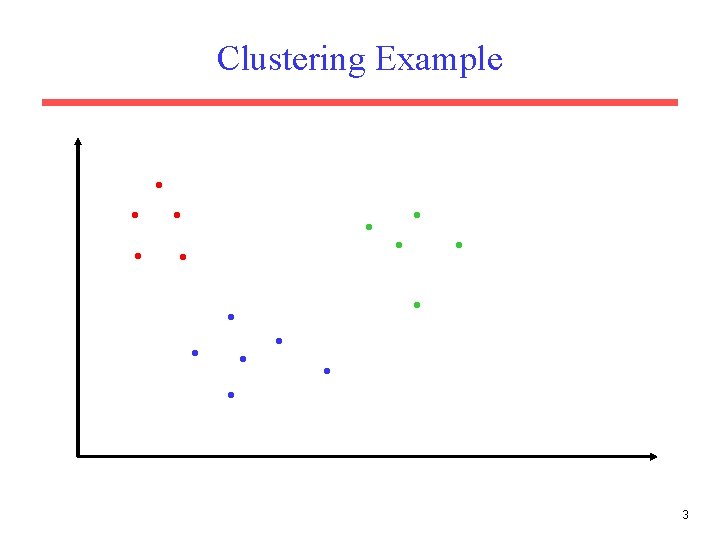
Clustering • Partition unlabeled examples into disjoint subsets of clusters, such that: – Examples within a cluster are very similar – Examples in different clusters are very different • Discover new categories in an unsupervised manner (no sample category labels provided). 2

Clustering Example . . . . 3

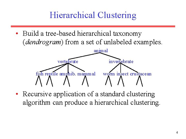
Hierarchical Clustering • Build a tree-based hierarchical taxonomy (dendrogram) from a set of unlabeled examples. animal vertebrate fish reptile amphib. mammal invertebrate worm insect crustacean • Recursive application of a standard clustering algorithm can produce a hierarchical clustering. 4

Aglommerative vs. Divisive Clustering • Aglommerative (bottom-up) methods start with each example in its own cluster and iteratively combine them to form larger and larger clusters. • Divisive (partitional, top-down) separate all examples immediately into clusters. 5

Direct Clustering Method • Direct clustering methods require a specification of the number of clusters, k, desired. • A clustering evaluation function assigns a real-value quality measure to a clustering. • The number of clusters can be determined automatically by explicitly generating clusterings for multiple values of k and choosing the best result according to a clustering evaluation function. 6

Hierarchical Agglomerative Clustering (HAC) • Assumes a similarity function for determining the similarity of two instances. • Starts with all instances in a separate cluster and then repeatedly joins the two clusters that are most similar until there is only one cluster. • The history of merging forms a binary tree or hierarchy. 7

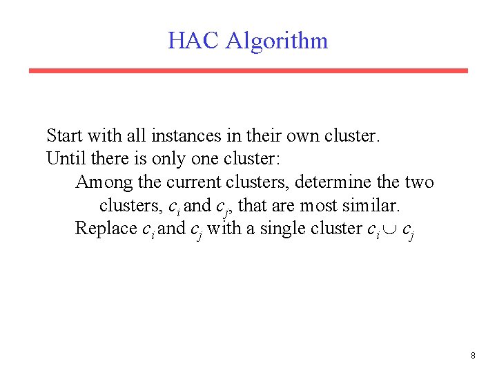
HAC Algorithm Start with all instances in their own cluster. Until there is only one cluster: Among the current clusters, determine the two clusters, ci and cj, that are most similar. Replace ci and cj with a single cluster ci cj 8

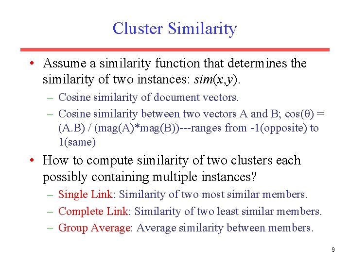
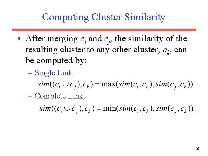
Cluster Similarity • Assume a similarity function that determines the similarity of two instances: sim(x, y). – Cosine similarity of document vectors. – Cosine similarity between two vectors A and B; cos(θ) = (A. B) / (mag(A)*mag(B))---ranges from -1(opposite) to 1(same) • How to compute similarity of two clusters each possibly containing multiple instances? – Single Link: Similarity of two most similar members. – Complete Link: Similarity of two least similar members. – Group Average: Average similarity between members. 9

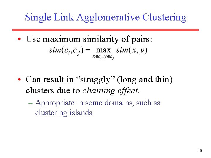
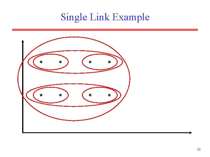
Single Link Agglomerative Clustering • Use maximum similarity of pairs: • Can result in “straggly” (long and thin) clusters due to chaining effect. – Appropriate in some domains, such as clustering islands. 10

Single Link Example 11

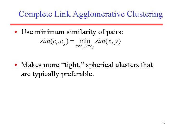
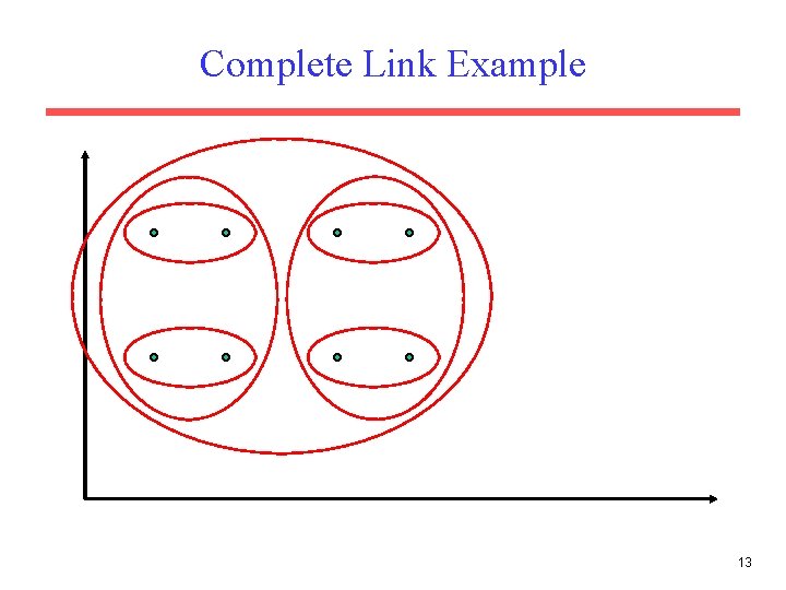
Complete Link Agglomerative Clustering • Use minimum similarity of pairs: • Makes more “tight, ” spherical clusters that are typically preferable. 12

Complete Link Example 13

Computational Complexity • In the first iteration, all HAC methods need to compute similarity of all pairs of n individual instances which is O(n 2). • In each of the subsequent n 2 merging iterations, it must compute the distance between the most recently created cluster and all other existing clusters. • In order to maintain an overall O(n 2) performance, computing similarity to each other cluster must be done in constant time. 14

Computing Cluster Similarity • After merging ci and cj, the similarity of the resulting cluster to any other cluster, ck, can be computed by: – Single Link: – Complete Link: 15

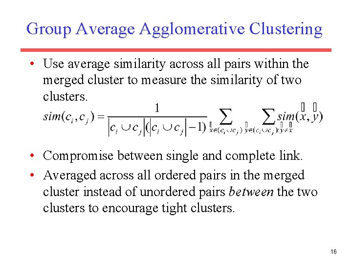
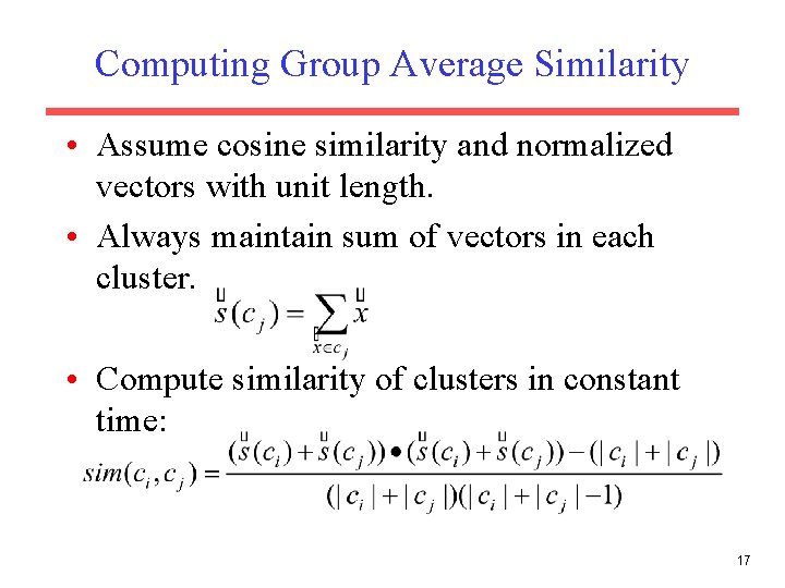
Group Average Agglomerative Clustering • Use average similarity across all pairs within the merged cluster to measure the similarity of two clusters. • Compromise between single and complete link. • Averaged across all ordered pairs in the merged cluster instead of unordered pairs between the two clusters to encourage tight clusters. 16

Computing Group Average Similarity • Assume cosine similarity and normalized vectors with unit length. • Always maintain sum of vectors in each cluster. • Compute similarity of clusters in constant time: 17

Non-Hierarchical Clustering • Typically must provide the number of desired clusters, k. • Randomly choose k instances as seeds, one per cluster. • Form initial clusters based on these seeds. • Iterate, repeatedly reallocating instances to different clusters to improve the overall clustering. • Stop when clustering converges or after a fixed number of iterations. 18

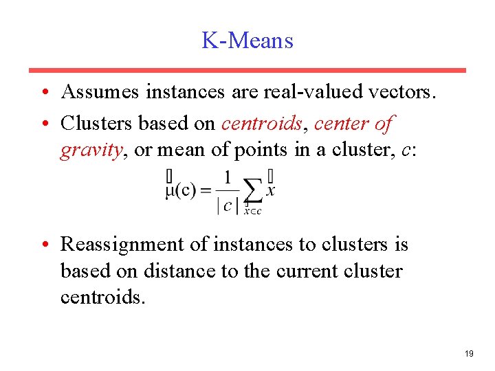
K-Means • Assumes instances are real-valued vectors. • Clusters based on centroids, center of gravity, or mean of points in a cluster, c: • Reassignment of instances to clusters is based on distance to the current cluster centroids. 19

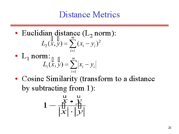
Distance Metrics • Euclidian distance (L 2 norm): • L 1 norm: • Cosine Similarity (transform to a distance by subtracting from 1): 20

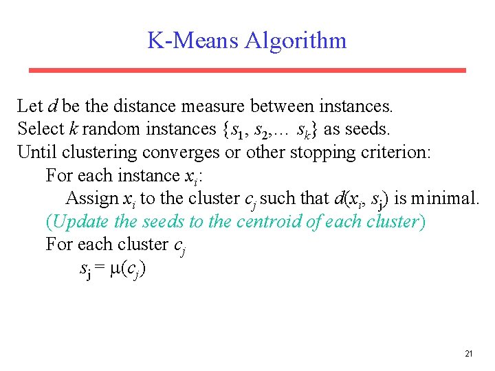
K-Means Algorithm Let d be the distance measure between instances. Select k random instances {s 1, s 2, … sk} as seeds. Until clustering converges or other stopping criterion: For each instance xi: Assign xi to the cluster cj such that d(xi, sj) is minimal. (Update the seeds to the centroid of each cluster) For each cluster cj sj = (cj) 21

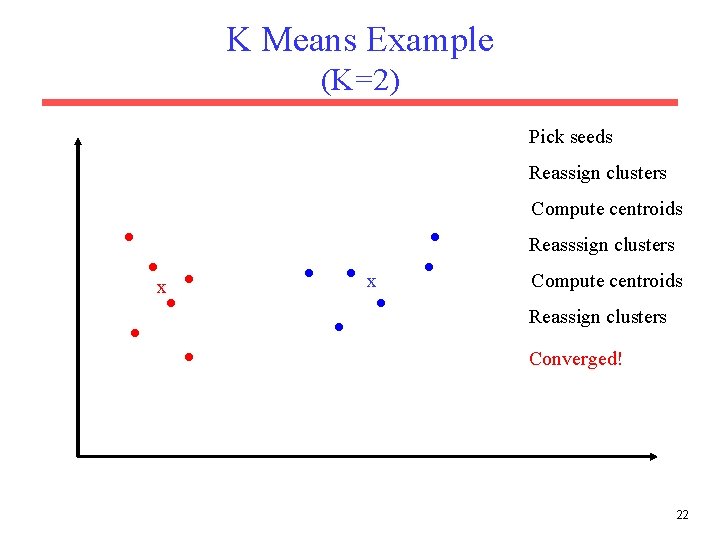
K Means Example (K=2) Pick seeds Reassign clusters Compute centroids Reasssign clusters x x Compute centroids Reassign clusters Converged! 22

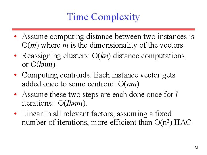
Time Complexity • Assume computing distance between two instances is O(m) where m is the dimensionality of the vectors. • Reassigning clusters: O(kn) distance computations, or O(knm). • Computing centroids: Each instance vector gets added once to some centroid: O(nm). • Assume these two steps are each done once for I iterations: O(Iknm). • Linear in all relevant factors, assuming a fixed number of iterations, more efficient than O(n 2) HAC. 23

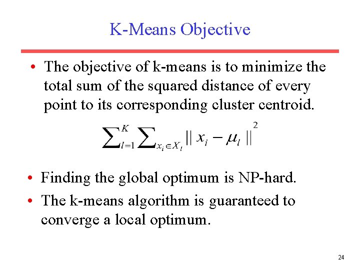
K-Means Objective • The objective of k-means is to minimize the total sum of the squared distance of every point to its corresponding cluster centroid. • Finding the global optimum is NP-hard. • The k-means algorithm is guaranteed to converge a local optimum. 24

Seed Choice • Results can vary based on random seed selection. • Some seeds can result in poor convergence rate, or convergence to sub-optimal clusterings. • Select good seeds using a heuristic or the results of another method. 25

Buckshot Algorithm • Combines HAC and K-Means clustering. • First randomly take a sample of instances of size n • Run group-average HAC on this sample, which takes only O(n) time. • Use the results of HAC as initial seeds for K -means. • Overall algorithm is O(n) and avoids problems of bad seed selection. 26

Text Clustering • HAC and K-Means have been applied to text in a straightforward way. • Typically use normalized, TF/IDF-weighted vectors and cosine similarity. • Optimize computations for sparse vectors. • Applications: – During retrieval, add other documents in the same cluster as the initial retrieved documents to improve recall. – Clustering of results of retrieval to present more organized results to the user (à la Northernlight folders). – Automated production of hierarchical taxonomies of documents for browsing purposes (à la Yahoo & DMOZ). 27

Soft Clustering • Clustering typically assumes that each instance is given a “hard” assignment to exactly one cluster. • Does not allow uncertainty in class membership or for an instance to belong to more than one cluster. • Soft clustering gives probabilities that an instance belongs to each of a set of clusters. • Each instance is assigned a probability distribution across a set of discovered categories (probabilities of all categories must sum to 1). 28

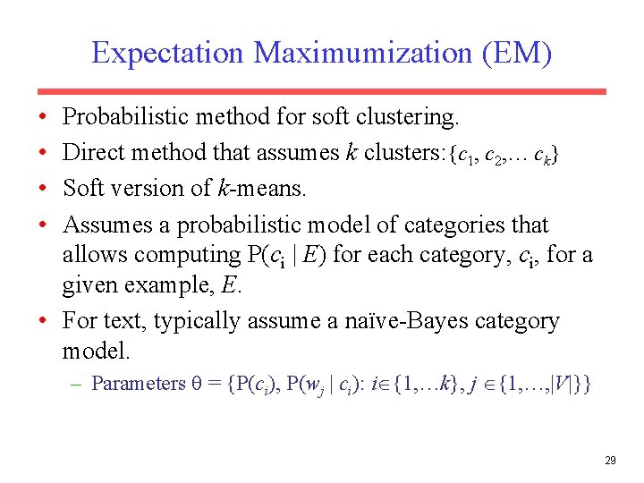
Expectation Maximumization (EM) • • Probabilistic method for soft clustering. Direct method that assumes k clusters: {c 1, c 2, … ck} Soft version of k-means. Assumes a probabilistic model of categories that allows computing P(ci | E) for each category, ci, for a given example, E. • For text, typically assume a naïve-Bayes category model. – Parameters = {P(ci), P(wj | ci): i {1, …k}, j {1, …, |V|}} 29

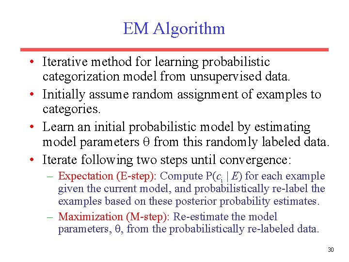
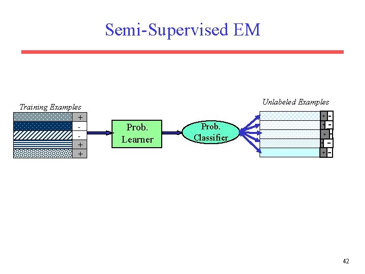
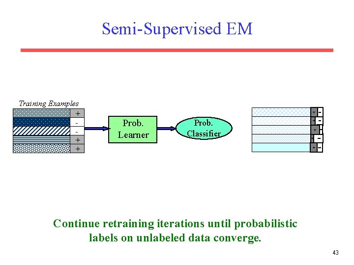
EM Algorithm • Iterative method for learning probabilistic categorization model from unsupervised data. • Initially assume random assignment of examples to categories. • Learn an initial probabilistic model by estimating model parameters from this randomly labeled data. • Iterate following two steps until convergence: – Expectation (E-step): Compute P(ci | E) for each example given the current model, and probabilistically re-label the examples based on these posterior probability estimates. – Maximization (M-step): Re-estimate the model parameters, , from the probabilistically re-labeled data. 30

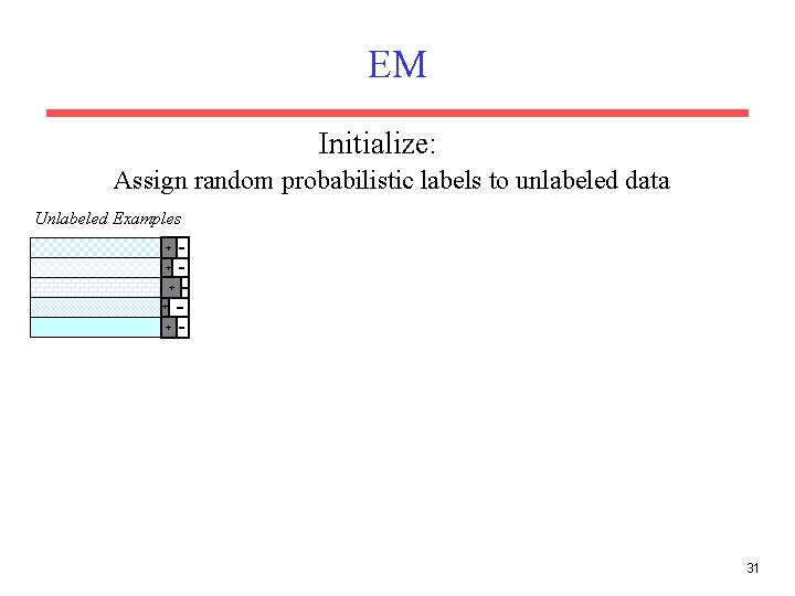
EM Initialize: Assign random probabilistic labels to unlabeled data Unlabeled Examples + + + 31

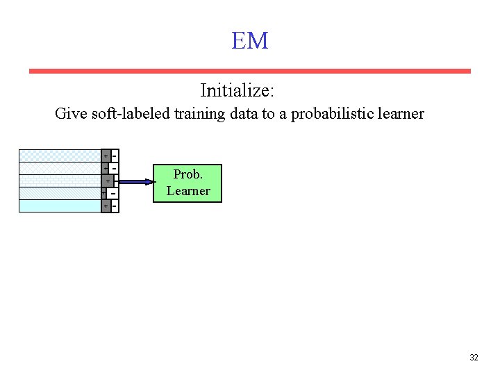
EM Initialize: Give soft-labeled training data to a probabilistic learner + + Prob. Learner + 32

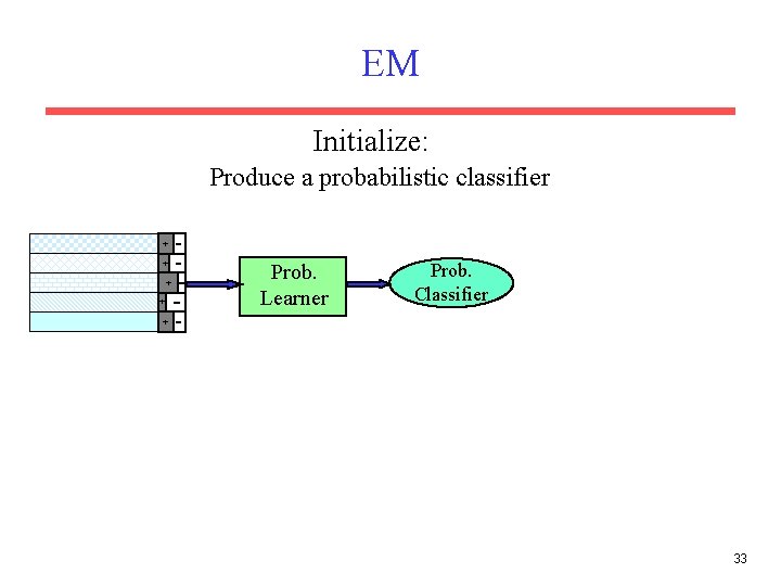
EM Initialize: Produce a probabilistic classifier + + Prob. Learner Prob. Classifier + 33

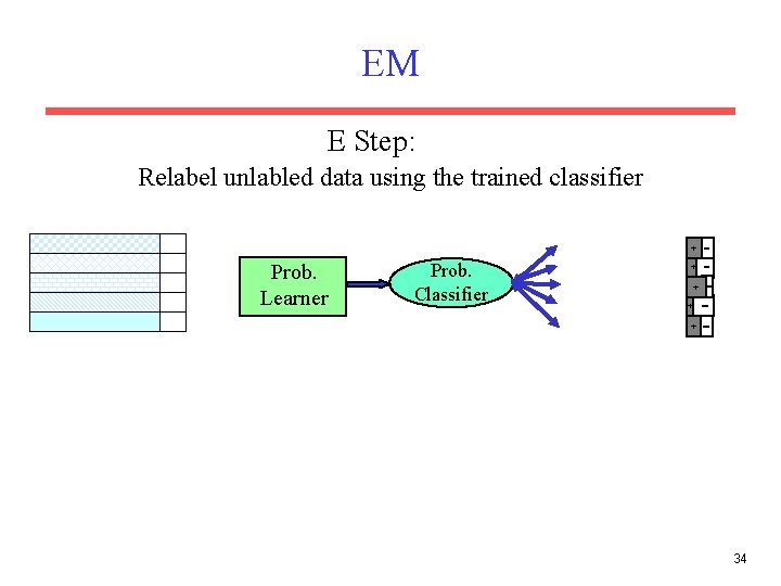
EM E Step: Relabel unlabled data using the trained classifier + Prob. Learner Prob. Classifier + + 34

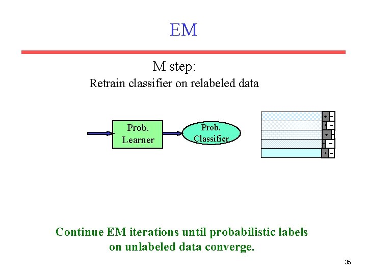
EM M step: Retrain classifier on relabeled data + Prob. Learner Prob. Classifier + + Continue EM iterations until probabilistic labels on unlabeled data converge. 35

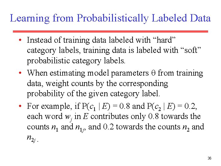
Learning from Probabilistically Labeled Data • Instead of training data labeled with “hard” category labels, training data is labeled with “soft” probabilistic category labels. • When estimating model parameters from training data, weight counts by the corresponding probability of the given category label. • For example, if P(c 1 | E) = 0. 8 and P(c 2 | E) = 0. 2, each word wj in E contributes only 0. 8 towards the counts n 1 and n 1 j, and 0. 2 towards the counts n 2 and n 2 j. 36

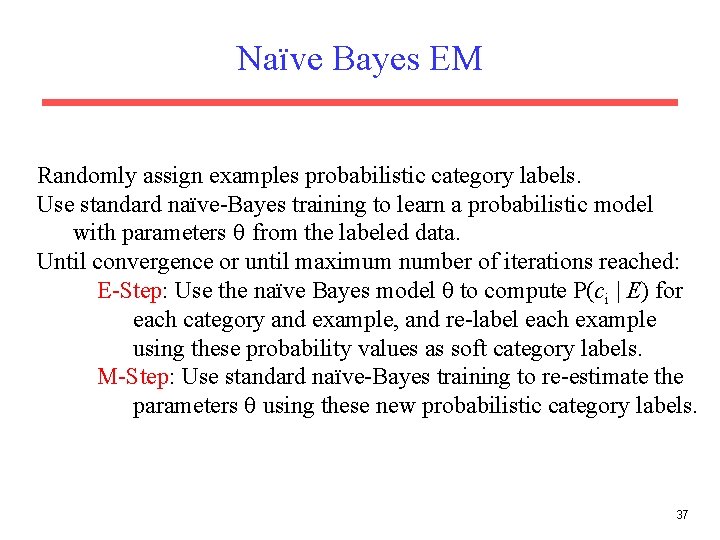
Naïve Bayes EM Randomly assign examples probabilistic category labels. Use standard naïve-Bayes training to learn a probabilistic model with parameters from the labeled data. Until convergence or until maximum number of iterations reached: E-Step: Use the naïve Bayes model to compute P(ci | E) for each category and example, and re-label each example using these probability values as soft category labels. M-Step: Use standard naïve-Bayes training to re-estimate the parameters using these new probabilistic category labels. 37

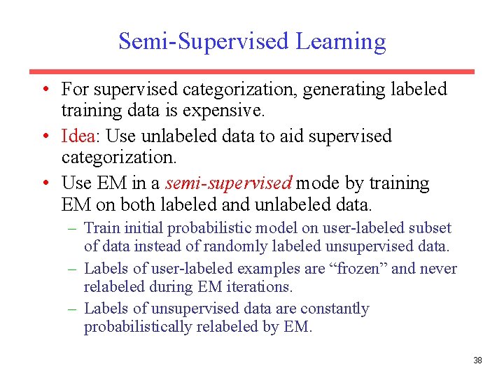
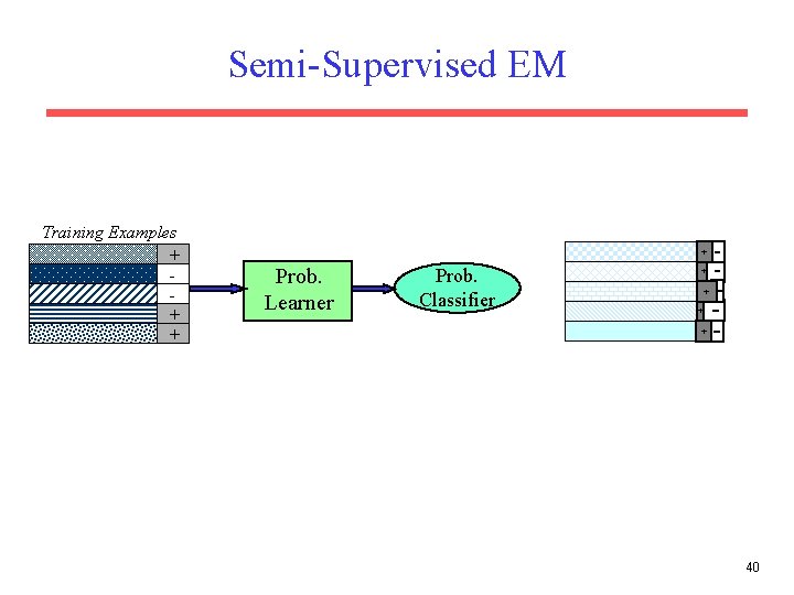
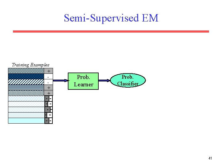
Semi-Supervised Learning • For supervised categorization, generating labeled training data is expensive. • Idea: Use unlabeled data to aid supervised categorization. • Use EM in a semi-supervised mode by training EM on both labeled and unlabeled data. – Train initial probabilistic model on user-labeled subset of data instead of randomly labeled unsupervised data. – Labels of user-labeled examples are “frozen” and never relabeled during EM iterations. – Labels of unsupervised data are constantly probabilistically relabeled by EM. 38

Semi-Supervised EM Training Examples + + + Unlabeled Examples + Prob. Learner Prob. Classifier + + 39

Semi-Supervised EM Training Examples + + Prob. Learner Prob. Classifier + + 40

Semi-Supervised EM Training Examples + + + Prob. Learner Prob. Classifier + + + 41

Semi-Supervised EM Training Examples + + + Unlabeled Examples + Prob. Learner Prob. Classifier + + 42

Semi-Supervised EM Training Examples + + Prob. Learner Prob. Classifier + + Continue retraining iterations until probabilistic labels on unlabeled data converge. 43

Semi-Supervised EM Results • Experiments on assigning messages from 20 Usenet newsgroups their proper newsgroup label. • With very few labeled examples (2 examples per class), semi-supervised EM significantly improved predictive accuracy: – 27% with 40 labeled messages only. – 43% with 40 labeled + 10, 000 unlabeled messages. • With more labeled examples, semi-supervision can actually decrease accuracy, but refinements to standard EM can help prevent this. – Must weight labeled data appropriately more than unlabeled data. • For semi-supervised EM to work, the “natural clustering of data” must be consistent with the desired categories – Failed when applied to English POS tagging (Merialdo, 1994) 44

Semi-Supervised EM Example • Assume “Catholic” is present in both of the labeled documents for soc. religion. christian, but “Baptist” occurs in none of the labeled data for this class. • From labeled data, we learn that “Catholic” is highly indicative of the “Christian” category. • When labeling unsupervised data, we label several documents with “Catholic” and “Baptist” correctly with the “Christian” category. • When retraining, we learn that “Baptist” is also indicative of a “Christian” document. • Final learned model is able to correctly assign documents containing only “Baptist” to “Christian”. 45

Issues in Unsupervised Learning • How to evaluate clustering? – Internal: • Tightness and separation of clusters (e. g. k-means objective) • Fit of probabilistic model to data – External • Compare to known class labels on benchmark data • • • Improving search to converge faster and avoid local minima. Overlapping clustering. Ensemble clustering. Clustering structured relational data. Semi-supervised methods other than EM: – Co-training – Transductive SVM’s – Semi-supervised clustering (must-link, cannot-link) 46

Conclusions • Unsupervised learning induces categories from unlabeled data. • There a variety of approaches, including: – HAC – k-means – EM • Semi-supervised learning uses both labeled and unlabeled data to improve results. 47