CS 3013 DS Algorithms Intro to Graph Algorithms

CS 3013: DS & Algorithms Intro to Graph Algorithms

Graphs l A graph G = (V, E) n n n V = set of vertices E = set of edges = subset of V V Thus |E| = O(|V|2)

Graph Variations l Variations: n n A connected graph has a path from every vertex to every other In an undirected graph: u Edge (u, v) = edge (v, u) u No self-loops n In a directed graph: u Edge (u, v) goes from vertex u to vertex v, notated u v

Graph Variations l More variations: n A weighted graph associates weights with either the edges or the vertices u E. g. , n a road map: edges might be weighted w/ distance A multigraph allows multiple edges between the same vertices u E. g. , the call graph in a program (a function can get called from multiple other functions)

Graphs l We will typically express running times in terms of |E| and |V| (often dropping the |’s) n n l If |E| |V|2 the graph is dense If |E| |V| the graph is sparse If you know you are dealing with dense or sparse graphs, different data structures may make sense

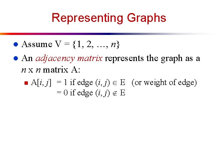
Representing Graphs Assume V = {1, 2, …, n} l An adjacency matrix represents the graph as a n x n matrix A: l n A[i, j] = 1 if edge (i, j) E (or weight of edge) = 0 if edge (i, j) E

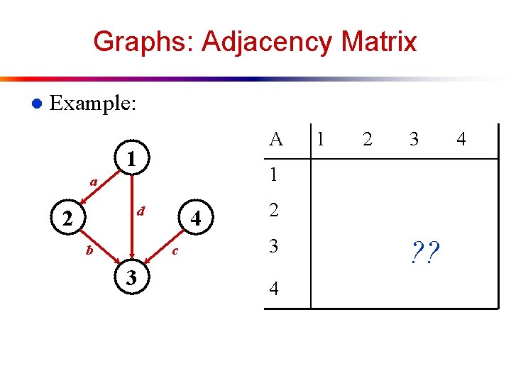
Graphs: Adjacency Matrix l Example: A 1 d b 4 c 3 2 3 1 a 2 1 2 3 4 ? ? 4

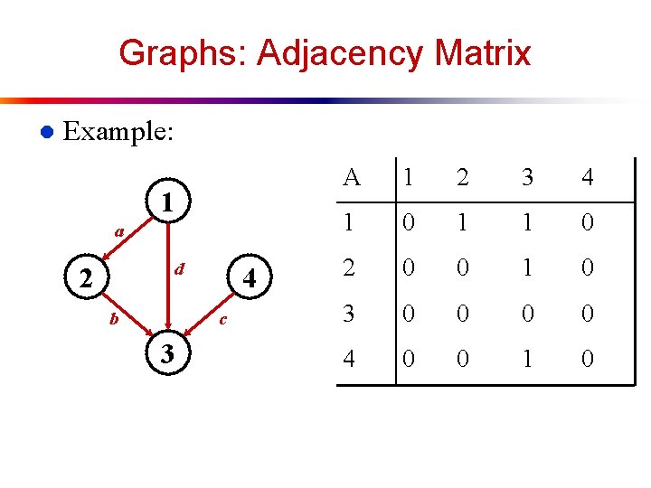
Graphs: Adjacency Matrix l Example: 1 a d 2 b 4 c 3 A 1 2 3 4 1 0 1 1 0 2 0 0 1 0 3 0 0 4 0 0 1 0

Graphs: Adjacency Matrix How much storage does the adjacency matrix require? l A: O(V 2) l What is the minimum amount of storage needed by an adjacency matrix representation of an undirected graph with 4 vertices? l A: 6 bits l n n Undirected graph matrix is symmetric No self-loops don’t need diagonal

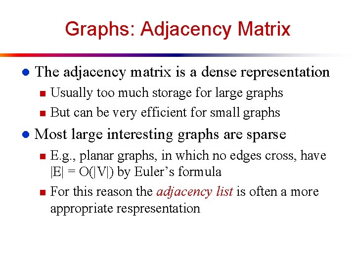
Graphs: Adjacency Matrix l The adjacency matrix is a dense representation n n l Usually too much storage for large graphs But can be very efficient for small graphs Most large interesting graphs are sparse n n E. g. , planar graphs, in which no edges cross, have |E| = O(|V|) by Euler’s formula For this reason the adjacency list is often a more appropriate respresentation

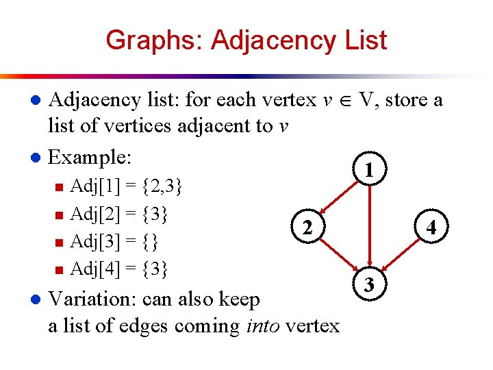
Graphs: Adjacency List Adjacency list: for each vertex v V, store a list of vertices adjacent to v l Example: 1 l n n l Adj[1] = {2, 3} Adj[2] = {3} Adj[3] = {} Adj[4] = {3} 2 Variation: can also keep a list of edges coming into vertex 4 3

Graphs: Adjacency List l How much storage is required? n The degree of a vertex v = # incident edges u Directed n n l graphs have in-degree, out-degree For directed graphs, # of items in adjacency lists is out-degree(v) = |E| takes (V + E) storage (Why? ) For undirected graphs, # items in adj lists is degree(v) = 2 |E| (handshaking lemma) also (V + E) storage So: Adjacency lists take O(V+E) storage

Graph Searching Given: a graph G = (V, E), directed or undirected l Goal: methodically explore every vertex and every edge l Ultimately: build a tree on the graph l n n n Pick a vertex as the root Choose certain edges to produce a tree Note: might also build a forest if graph is not connected

Breadth-First Search l “Explore” a graph, turning it into a tree n n l One vertex at a time Expand frontier of explored vertices across the breadth of the frontier Builds a tree over the graph n n Pick a source vertex to be the root Find (“discover”) its children, then their children, etc.

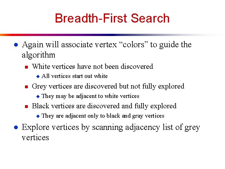
Breadth-First Search l Again will associate vertex “colors” to guide the algorithm n White vertices have not been discovered u n Grey vertices are discovered but not fully explored u n They may be adjacent to white vertices Black vertices are discovered and fully explored u l All vertices start out white They are adjacent only to black and gray vertices Explore vertices by scanning adjacency list of grey vertices

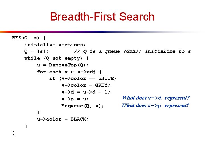
Breadth-First Search BFS(G, s) { initialize vertices; Q = {s}; // Q is a queue (duh); initialize to s while (Q not empty) { u = Remove. Top(Q); for each v u->adj { if (v->color == WHITE) v->color = GREY; v->d = u->d + 1; What does v->d represent? v->p = u; Enqueue(Q, v); What does v->p represent? } u->color = BLACK; } }

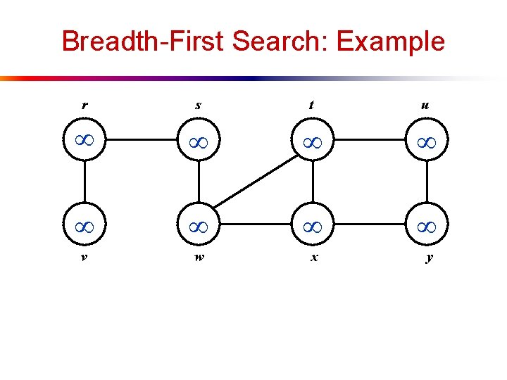
Breadth-First Search: Example r s t u v w x y

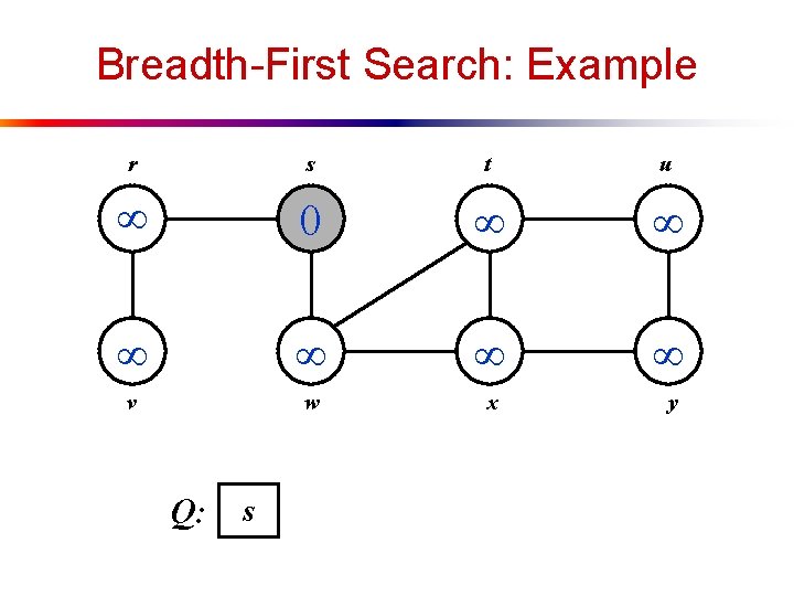
Breadth-First Search: Example r s t u 0 v w x y Q: s

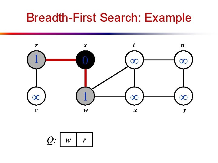
Breadth-First Search: Example r s t u 1 0 1 v w x y Q: w r

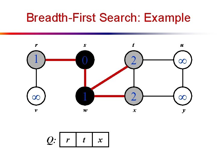
Breadth-First Search: Example r s t u 1 0 2 1 2 v w x y Q: r t x

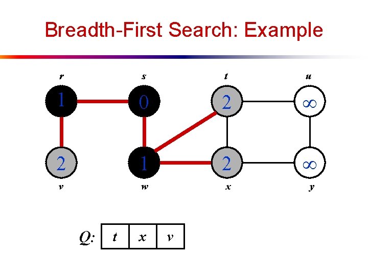
Breadth-First Search: Example r s t u 1 0 2 2 1 2 v w x y Q: t x v

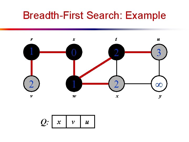
Breadth-First Search: Example r s t u 1 0 2 3 2 1 2 v w x y Q: x v u

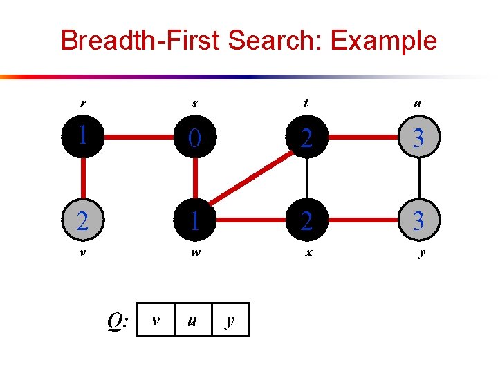
Breadth-First Search: Example r s t u 1 0 2 3 2 1 2 3 v w x y Q: v u y

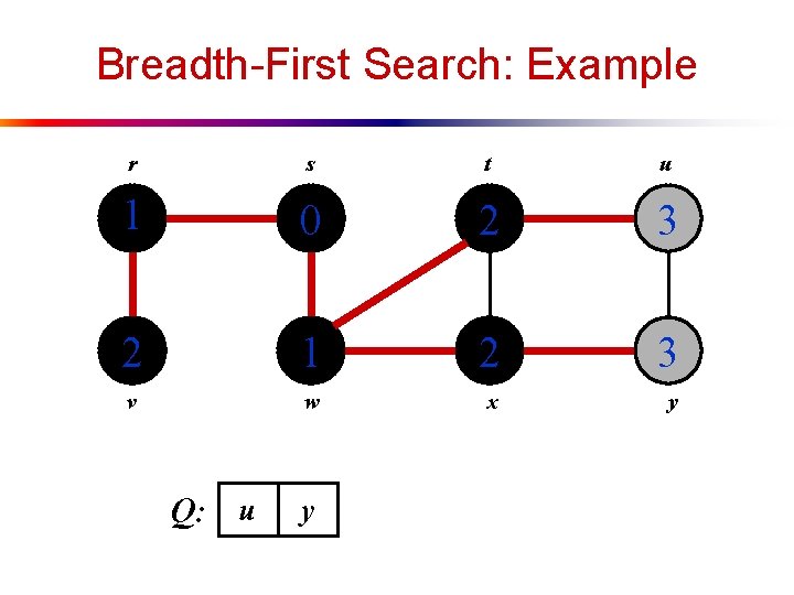
Breadth-First Search: Example r s t u 1 0 2 3 2 1 2 3 v w x y Q: u y

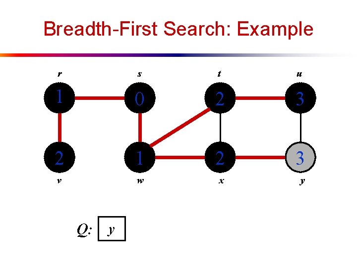
Breadth-First Search: Example r s t u 1 0 2 3 2 1 2 3 v w x y Q: y

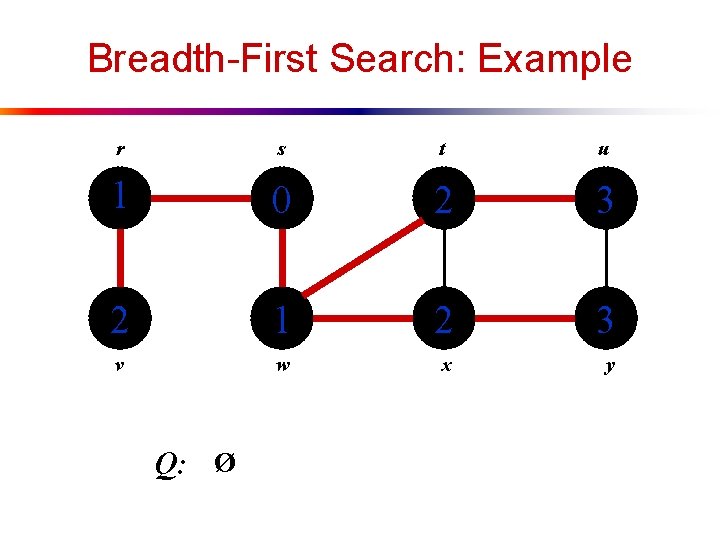
Breadth-First Search: Example r s t u 1 0 2 3 2 1 2 3 v w x y Q: Ø

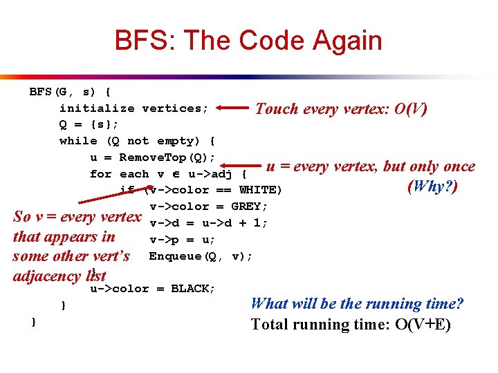
BFS: The Code Again BFS(G, s) { initialize vertices; Touch every vertex: O(V) Q = {s}; while (Q not empty) { u = Remove. Top(Q); for each v u->adj { u = every vertex, but only once (Why? ) if (v->color == WHITE) v->color = GREY; So v = every vertex v->d = u->d + 1; that appears in v->p = u; some other vert’s Enqueue(Q, v); } adjacency list u->color = BLACK; What will be the running time? } } Total running time: O(V+E)

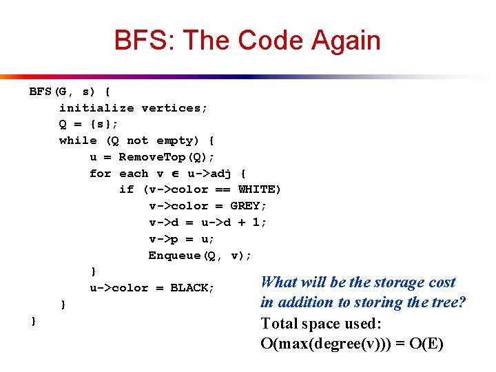
BFS: The Code Again BFS(G, s) { initialize vertices; Q = {s}; while (Q not empty) { u = Remove. Top(Q); for each v u->adj { if (v->color == WHITE) v->color = GREY; v->d = u->d + 1; v->p = u; Enqueue(Q, v); } What will be the storage cost u->color = BLACK; in addition to storing the tree? } } Total space used: O(max(degree(v))) = O(E)

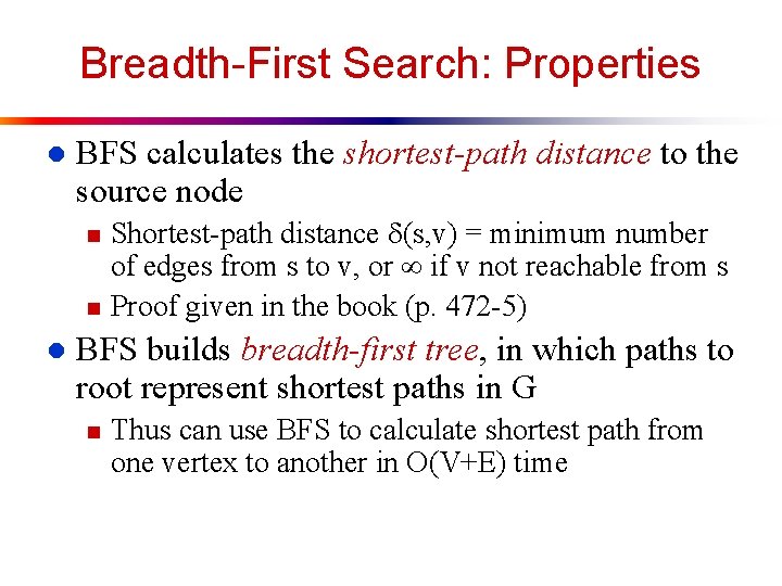
Breadth-First Search: Properties l BFS calculates the shortest-path distance to the source node n n l Shortest-path distance (s, v) = minimum number of edges from s to v, or if v not reachable from s Proof given in the book (p. 472 -5) BFS builds breadth-first tree, in which paths to root represent shortest paths in G n Thus can use BFS to calculate shortest path from one vertex to another in O(V+E) time

Depth-First Search l Depth-first search is another strategy for exploring a graph n n n Explore “deeper” in the graph whenever possible Edges are explored out of the most recently discovered vertex v that still has unexplored edges When all of v’s edges have been explored, backtrack to the vertex from which v was discovered

Depth-First Search Vertices initially colored white l Then colored gray when discovered l Then black when finished l

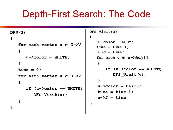
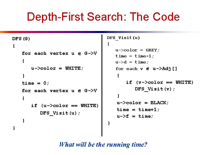
Depth-First Search: The Code DFS(G) { for each vertex u G->V { u->color = WHITE; } time = 0; for each vertex u G->V { if (u->color == WHITE) DFS_Visit(u); } } DFS_Visit(u) { u->color = GREY; time = time+1; u->d = time; for each v u->Adj[] { if (v->color == WHITE) DFS_Visit(v); } u->color = BLACK; time = time+1; u->f = time; }

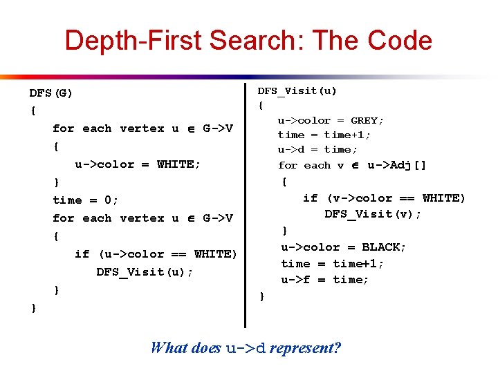
Depth-First Search: The Code DFS(G) { for each vertex u G->V { u->color = WHITE; } time = 0; for each vertex u G->V { if (u->color == WHITE) DFS_Visit(u); } } DFS_Visit(u) { u->color = GREY; time = time+1; u->d = time; for each v u->Adj[] { if (v->color == WHITE) DFS_Visit(v); } u->color = BLACK; time = time+1; u->f = time; } What does u->d represent?

Depth-First Search: The Code DFS(G) { for each vertex u G->V { u->color = WHITE; } time = 0; for each vertex u G->V { if (u->color == WHITE) DFS_Visit(u); } } DFS_Visit(u) { u->color = GREY; time = time+1; u->d = time; for each v u->Adj[] { if (v->color == WHITE) DFS_Visit(v); } u->color = BLACK; time = time+1; u->f = time; } What does u->f represent?

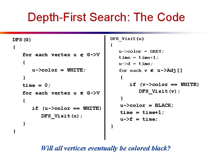
Depth-First Search: The Code DFS(G) { for each vertex u G->V { u->color = WHITE; } time = 0; for each vertex u G->V { if (u->color == WHITE) DFS_Visit(u); } } DFS_Visit(u) { u->color = GREY; time = time+1; u->d = time; for each v u->Adj[] { if (v->color == WHITE) DFS_Visit(v); } u->color = BLACK; time = time+1; u->f = time; } Will all vertices eventually be colored black?

Depth-First Search: The Code DFS(G) { for each vertex u G->V { u->color = WHITE; } time = 0; for each vertex u G->V { if (u->color == WHITE) DFS_Visit(u); } } DFS_Visit(u) { u->color = GREY; time = time+1; u->d = time; for each v u->Adj[] { if (v->color == WHITE) DFS_Visit(v); } u->color = BLACK; time = time+1; u->f = time; } What will be the running time?

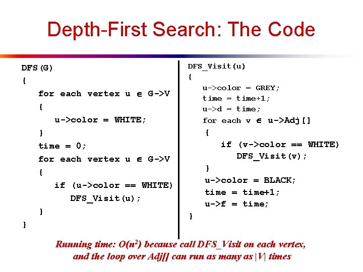
Depth-First Search: The Code DFS(G) { for each vertex u G->V { u->color = WHITE; } time = 0; for each vertex u G->V { if (u->color == WHITE) DFS_Visit(u); } } DFS_Visit(u) { u->color = GREY; time = time+1; u->d = time; for each v u->Adj[] { if (v->color == WHITE) DFS_Visit(v); } u->color = BLACK; time = time+1; u->f = time; } Running time: O(n 2) because call DFS_Visit on each vertex, and the loop over Adj[] can run as many as |V| times

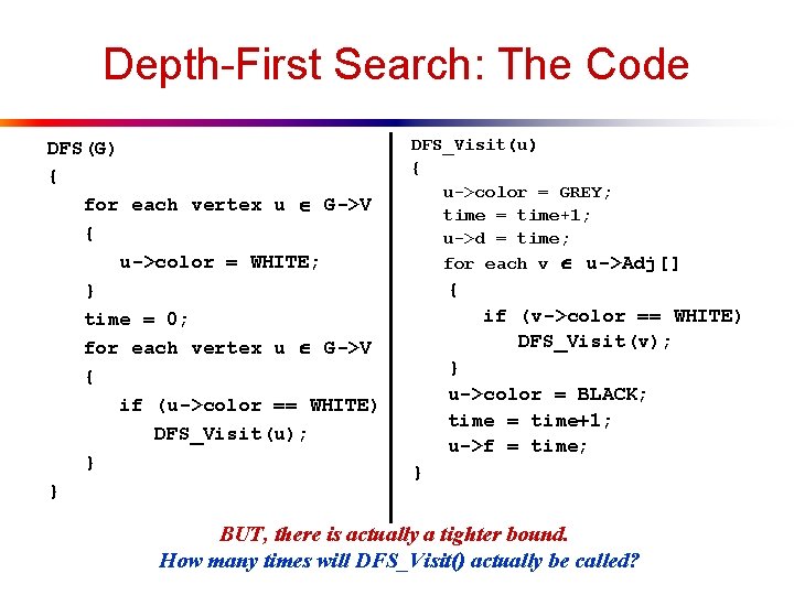
Depth-First Search: The Code DFS(G) { for each vertex u G->V { u->color = WHITE; } time = 0; for each vertex u G->V { if (u->color == WHITE) DFS_Visit(u); } } DFS_Visit(u) { u->color = GREY; time = time+1; u->d = time; for each v u->Adj[] { if (v->color == WHITE) DFS_Visit(v); } u->color = BLACK; time = time+1; u->f = time; } BUT, there is actually a tighter bound. How many times will DFS_Visit() actually be called?

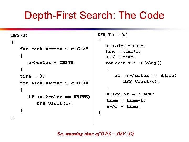
Depth-First Search: The Code DFS(G) { for each vertex u G->V { u->color = WHITE; } time = 0; for each vertex u G->V { if (u->color == WHITE) DFS_Visit(u); } } DFS_Visit(u) { u->color = GREY; time = time+1; u->d = time; for each v u->Adj[] { if (v->color == WHITE) DFS_Visit(v); } u->color = BLACK; time = time+1; u->f = time; } So, running time of DFS = O(V+E)

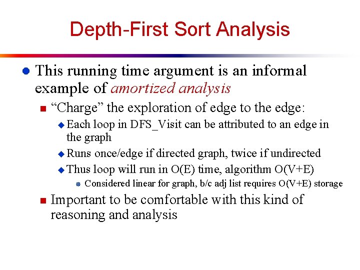
Depth-First Sort Analysis l This running time argument is an informal example of amortized analysis n “Charge” the exploration of edge to the edge: u Each loop in DFS_Visit can be attributed to an edge in the graph u Runs once/edge if directed graph, twice if undirected u Thus loop will run in O(E) time, algorithm O(V+E) ] n Considered linear for graph, b/c adj list requires O(V+E) storage Important to be comfortable with this kind of reasoning and analysis

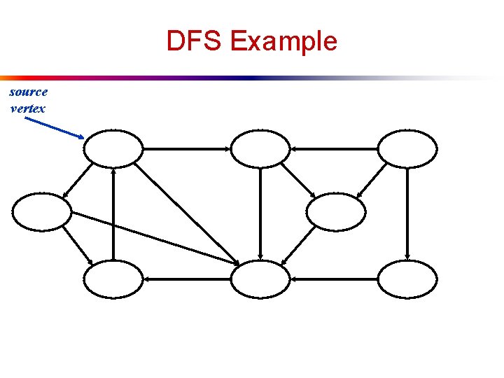
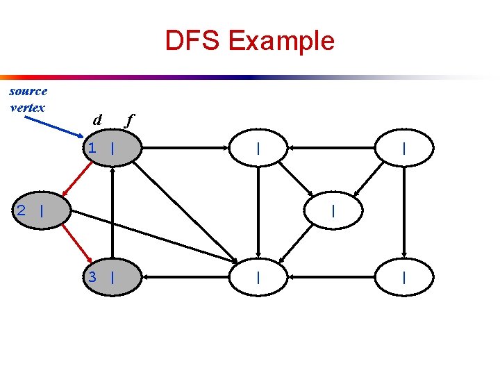
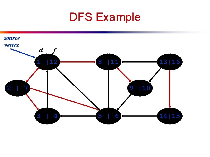
DFS Example source vertex

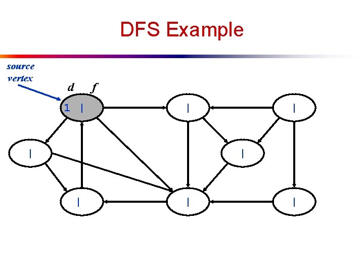
DFS Example source vertex d f 1 | | | |

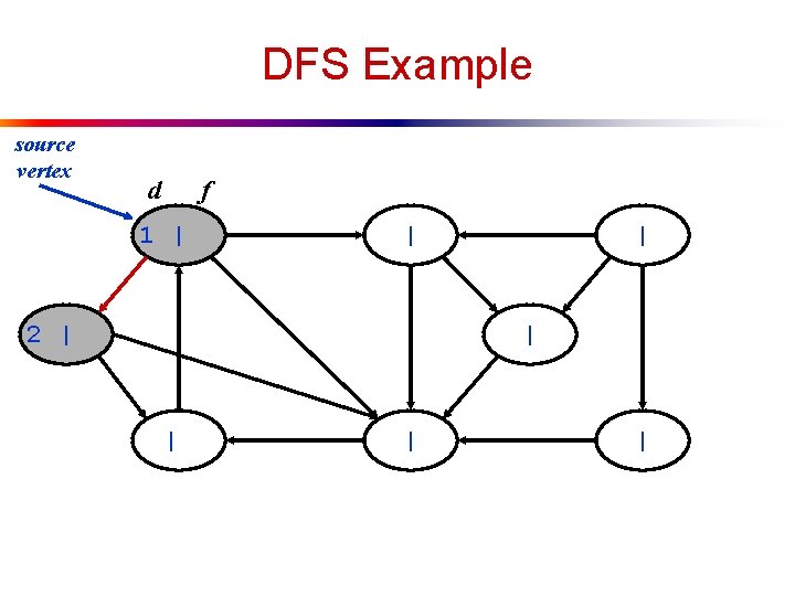
DFS Example source vertex d f 1 | | 2 | | |

DFS Example source vertex d 1 | f | 2 | | | 3 | | |

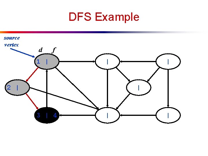
DFS Example source vertex d f 1 | | 2 | | | 3 | 4 | |

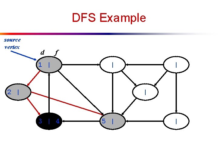
DFS Example source vertex d f 1 | | 2 | | | 3 | 4 5 | |

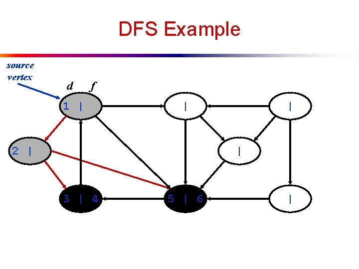
DFS Example source vertex d f 1 | | 2 | | | 3 | 4 5 | 6 |

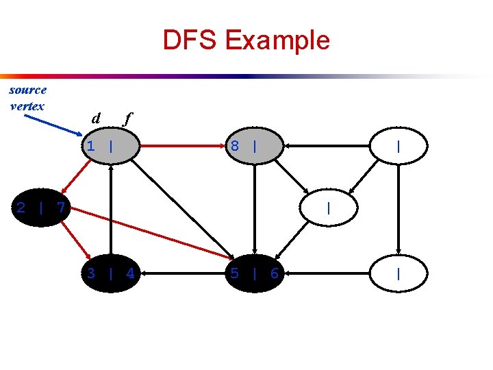
DFS Example source vertex d f 1 | 8 | 2 | 7 | | 3 | 4 5 | 6 |

DFS Example source vertex d f 1 | 8 | 2 | 7 | | 3 | 4 5 | 6 |

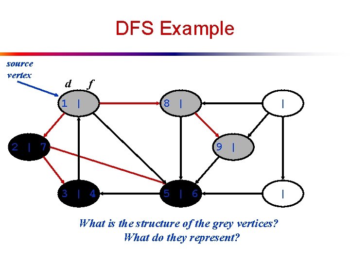
DFS Example source vertex d f 1 | 8 | 2 | 7 | 9 | 3 | 4 5 | 6 What is the structure of the grey vertices? What do they represent? |

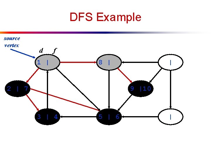
DFS Example source vertex d f 1 | 8 | 2 | 7 | 9 |10 3 | 4 5 | 6 |

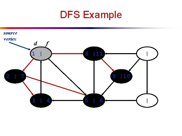
DFS Example source vertex d f 1 | 8 |11 2 | 7 | 9 |10 3 | 4 5 | 6 |

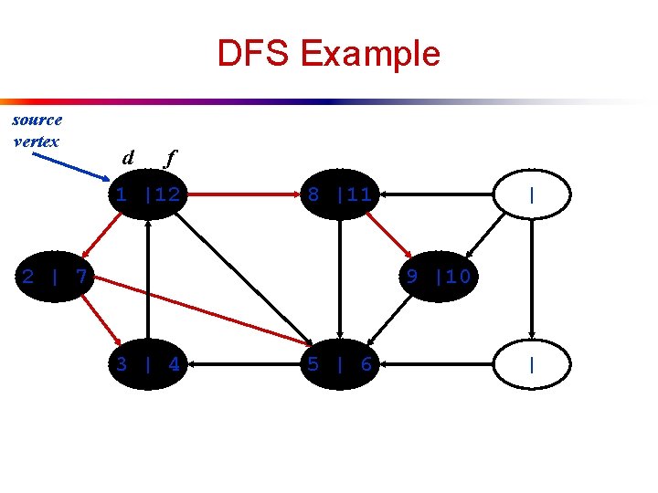
DFS Example source vertex d f 1 |12 8 |11 2 | 7 | 9 |10 3 | 4 5 | 6 |

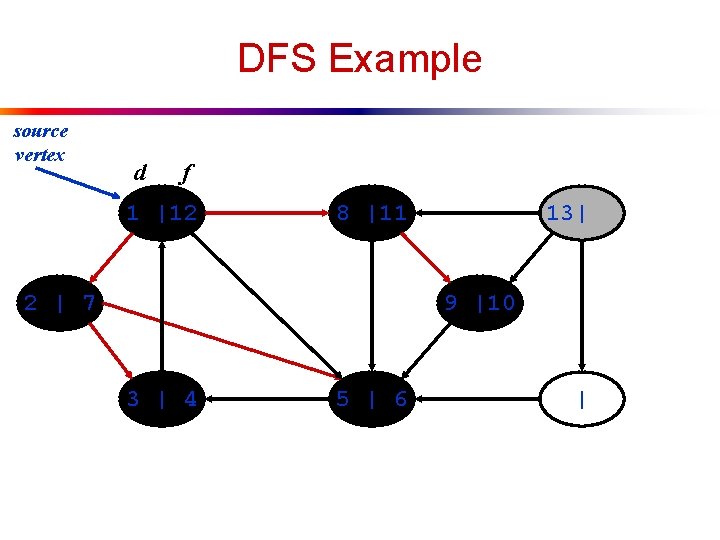
DFS Example source vertex d f 1 |12 8 |11 2 | 7 13| 9 |10 3 | 4 5 | 6 |

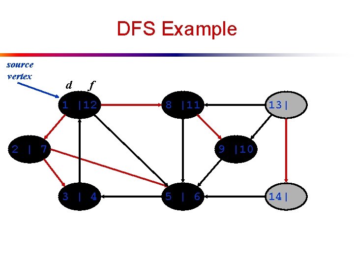
DFS Example source vertex d f 1 |12 8 |11 2 | 7 13| 9 |10 3 | 4 5 | 6 14|

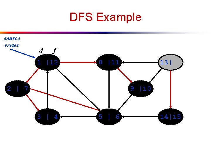
DFS Example source vertex d f 1 |12 8 |11 2 | 7 13| 9 |10 3 | 4 5 | 6 14|15

DFS Example source vertex d f 1 |12 8 |11 2 | 7 13|16 9 |10 3 | 4 5 | 6 14|15

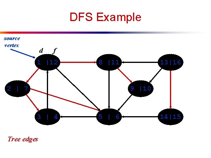
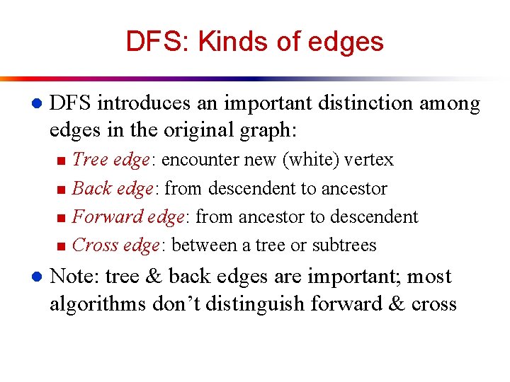
DFS: Kinds of edges l DFS introduces an important distinction among edges in the original graph: n Tree edge: encounter new (white) vertex u The tree edges form a spanning forest u Can tree edges form cycles? Why or why not?

DFS Example source vertex d f 1 |12 8 |11 2 | 7 13|16 9 |10 3 | 4 Tree edges 5 | 6 14|15

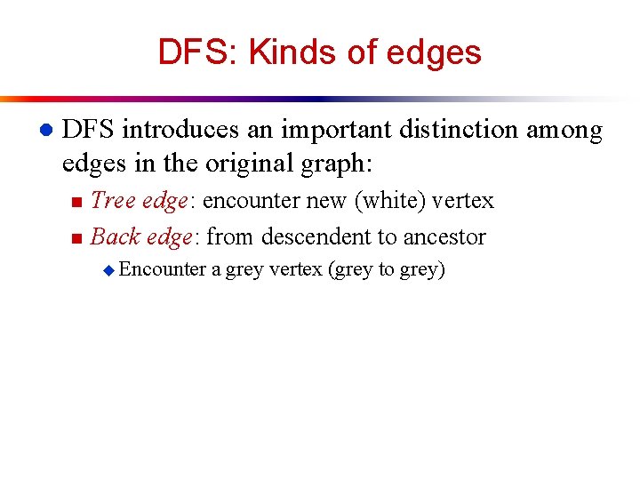
DFS: Kinds of edges l DFS introduces an important distinction among edges in the original graph: n n Tree edge: encounter new (white) vertex Back edge: from descendent to ancestor u Encounter a grey vertex (grey to grey)

DFS Example source vertex d f 1 |12 8 |11 2 | 7 13|16 9 |10 3 | 4 Tree edges Back edges 5 | 6 14|15

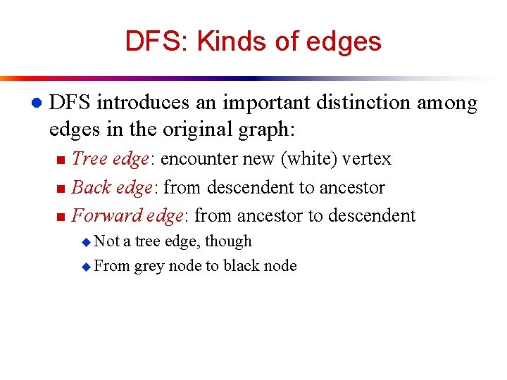
DFS: Kinds of edges l DFS introduces an important distinction among edges in the original graph: n n n Tree edge: encounter new (white) vertex Back edge: from descendent to ancestor Forward edge: from ancestor to descendent u Not a tree edge, though u From grey node to black node

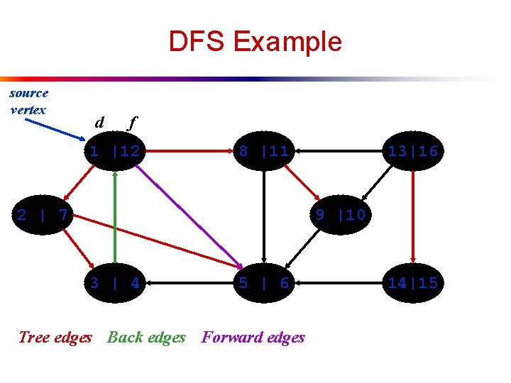
DFS Example source vertex d f 1 |12 8 |11 2 | 7 13|16 9 |10 3 | 4 5 | 6 Tree edges Back edges Forward edges 14|15

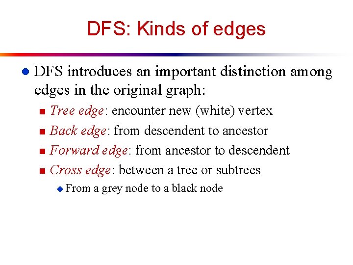
DFS: Kinds of edges l DFS introduces an important distinction among edges in the original graph: n n Tree edge: encounter new (white) vertex Back edge: from descendent to ancestor Forward edge: from ancestor to descendent Cross edge: between a tree or subtrees u From a grey node to a black node

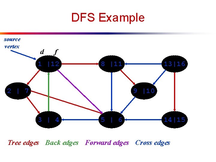
DFS Example source vertex d f 1 |12 8 |11 2 | 7 13|16 9 |10 3 | 4 5 | 6 14|15 Tree edges Back edges Forward edges Cross edges

DFS: Kinds of edges l DFS introduces an important distinction among edges in the original graph: n n l Tree edge: encounter new (white) vertex Back edge: from descendent to ancestor Forward edge: from ancestor to descendent Cross edge: between a tree or subtrees Note: tree & back edges are important; most algorithms don’t distinguish forward & cross

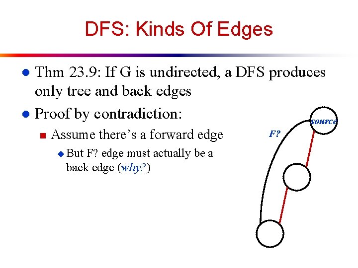
DFS: Kinds Of Edges Thm 23. 9: If G is undirected, a DFS produces only tree and back edges l Proof by contradiction: source l n Assume there’s a forward edge u But F? edge must actually be a back edge (why? ) F?

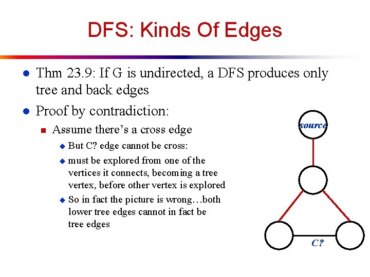
DFS: Kinds Of Edges l l Thm 23. 9: If G is undirected, a DFS produces only tree and back edges Proof by contradiction: n Assume there’s a cross edge source But C? edge cannot be cross: u must be explored from one of the vertices it connects, becoming a tree vertex, before other vertex is explored u So in fact the picture is wrong…both lower tree edges cannot in fact be tree edges u C?

DFS And Graph Cycles l Thm: An undirected graph is acyclic iff a DFS yields no back edges n n If acyclic, no back edges (because a back edge implies a cycle If no back edges, acyclic No back edges implies only tree edges (Why? ) u Only tree edges implies we have a tree or a forest u Which by definition is acyclic u l Thus, can run DFS to find whether a graph has a cycle

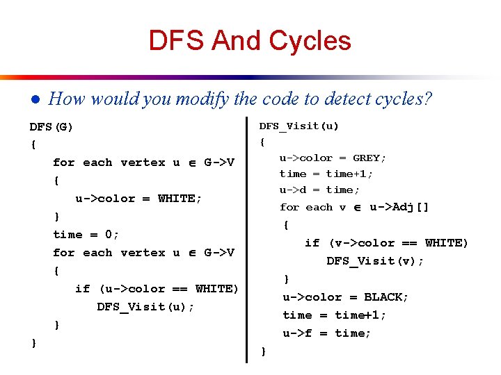
DFS And Cycles l How would you modify the code to detect cycles? DFS(G) { for each vertex u G->V { u->color = WHITE; } time = 0; for each vertex u G->V { if (u->color == WHITE) DFS_Visit(u); } } DFS_Visit(u) { u->color = GREY; time = time+1; u->d = time; for each v u->Adj[] { if (v->color == WHITE) DFS_Visit(v); } u->color = BLACK; time = time+1; u->f = time; }

DFS And Cycles l What will be the running time? DFS(G) { for each vertex u G->V { u->color = WHITE; } time = 0; for each vertex u G->V { if (u->color == WHITE) DFS_Visit(u); } } DFS_Visit(u) { u->color = GREY; time = time+1; u->d = time; for each v u->Adj[] { if (v->color == WHITE) DFS_Visit(v); } u->color = BLACK; time = time+1; u->f = time; }

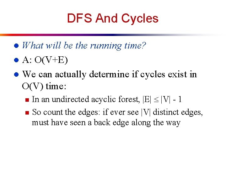
DFS And Cycles What will be the running time? l A: O(V+E) l We can actually determine if cycles exist in O(V) time: l n n In an undirected acyclic forest, |E| |V| - 1 So count the edges: if ever see |V| distinct edges, must have seen a back edge along the way

The End