CS 294 43 Multiple Kernel and Segmentation methods

Last Lecture – Category Discovery • R. Fergus, L. Fei-Fei, P. Perona, and A.

Today – Kernel Combination, Segmentation, and Structured Output • M. Varma and D. Ray,

Multiple Kernel Learning Manik Varma Microsoft Research India Alex Berg, Anna Bosch, Varun Gulshan,

SVMs and MKL • SVMs are basic tools in machine learning that can be

Object Categorization Chair Schooner ? = Ketch Novel image to be classified Taj Panda

Outline of the Talk • Introduction to SVMs and kernel learning. • Our Multiple

Introduction to SVMs and Kernel Learning

Binary Classification With SVMs K(xi, xj) = t(xi) (xj) Margin = 2 / wtw

The C-SVM Primal Formulation • Minimisew, b, ½wtw + C i i • Subject

The C-SVM Dual Formulation • Maximise 1 t – ½ t. YKY • Subject

Some Popular Kernels • Linear: K(xi, xj) = xit -1 xj t -1 x

Advantages of Learning the Kernel • Learn the kernel parameters • Improve accuracy and

Linear Combinations of Base Kernels • Learn a linear combination of base kernels •

Linear Combinations of Base Kernels Schooner Ketch Simplistic 1 D colour feature c •

Linear Combinations of Base Kernels Schooner Ketch Simplistic 1 D shape feature s •

Linear Combinations of Base Kernels • We learn a combined colour-shape feature space. •

Multiple Kernel Learning [Varma & Ray 07] NP Hard Region d 2 d ≥

Multiple Kernel Learning Primal Formulation • Minimisew, b, , d ½wtw + C i

Multiple Kernel Learning Dual Formulation • Maximise 1 t • Subject to • 0≤

Large Scale Reformulation • Minimised T(d) subject to d ≥ 0 • where T(d)

Large Scale Reformulation Contour plot of T(d) Surface plot of -T(d) • We turn

Dual - Differentiability • W(d) = Max 1 t + td – ½ k

Dual - Derivative • W(d) = Max 1 t + td – ½ k

Final Algorithm 1. Initialise d 0 randomly 2. Repeat until convergence a) Form K(x,

The Caltech 101 Database • Object category database collected by Fei-Fei et al. [PAMI

Caltech 101 – Experimental Setup • Experimental setup kept identical to that of Zhang

Experimental Results – Caltech 101 1 -NN SVM (1 -vs-1) SVM (1 -vs-All) Shape

Extending Our MKL Formulation • Minimisew, b, d ½wtw + i L(f(xi), yi) +

Kernel Generalizations • The learnt kernel can now have any functional form as long

Regularization Generalizations • Any regulariser can be used as long as it has continuous

Loss Function Generalizations • The loss function can be generalized to handle • Regression.

Multiple Kernel Regression Formulation • Minimisew, b, d ½wtw + C i i +

Probabilistic Interpretation for Regression • MAP estimation with the following priors and likelihood p(b)

Predicting Facial Attractiveness Anandan Chris What is their rating on the milli. Helen scale?

Regression on Hot or Not Training Data 7. 3 8. 7 6. 5 6.

Predicting Facial Attractiveness – Features • Geometric features: Face, eyes, nose and lip contours.

Predicting Facial Attractiveness Francis Bach 8. 85 Luc Van Gool Phil Torr 8. 58

Recognition using Regions Chunhui Gu, Joseph Lim, Pablo Arbelaez, Jitendra Malik UC Berkeley

Grand Recognition Problem • Detection • Segmentation Tiger • Classification

Region Extraction Region Segmentation Bag of Regions

Weight Learning • Not all regions are equally important DIK DIJ image J exemplar

Detection/Segmentation Algorithm Exemplars Detection Images Verification classifier Ground truths Region matching based voting Query

Verification • For exemplar 1, 2, …, N of class C, define likelihood function

Segmentation Query Initial Seeds Exemplar Constrained Mask Result

ETHZ Shape (Ferrari et al. 06) • Contains 255 images of 5 diverse shape‐based

Detection/Segmentation Results • Significantly outperforms the state of the art (Ferrari et al. CVPR

Caltech 101 (Fei‐Fei et al. 04) • 102 classes, 31‐ 800 images/class

Conclusion • Introduce a unified framework for object detection, segmentation and classification • Regions

Multiplicative kernels for parameterized detectors Object Detection (binary classification) Umm, this doesn’t look like

Proposed Approach We try to learn a function which tells whether is an instance

Why If we fix , - intuitions is a detector of a specific Parameter

Learning of function C Assume C can be factorized into a feature space mapping

Approximation of W is approximated by basis function expansion: where vectors are unknowns and

Kernel Representation If we plug and The unknowns are in . into is the

Kernel Representation If we solve the binary classification problem by SVM, the actual kernel

Kernel Representation After SVM learning, the classification function becomes where is the weight of

Short Summary We have a way to learn evaluates tuples. which corresponds to a

Training Process Each training sample is in the form of a tuple x 1

Feasibility Experiment III Vehicle data set, 12 view categories. Learning a Family of Detectors,

Feasibility Experiment III is an RBF kernel defined with Euclidean distance in HOG space

Feasibility Experiment III Vehicle view angle estimation (multi-classification) Baseline method (12 subclass detectors): 62.

Next Lecture – Image Context • A. Torralba, K. P. Murphy, and W. T.

Slides: 98

Download presentation

CS 294‐ 43: Multiple Kernel and Segmentation methods Prof. Trevor Darrell Spring 2009 April 7 th , 2009

Last Lecture – Category Discovery • R. Fergus, L. Fei-Fei, P. Perona, and A. Zisserman, "Learning object categories from google's image search, " ICCV vol. 2, 2005 • L. -J. Li, G. Wang, and L. Fei-Fei, "Optimol: automatic online picture collection via incremental model learning, " in Computer Vision and Pattern Recognition, 2007. CVPR '07 • F. Schroff, A. Criminisi, and A. Zisserman, "Harvesting image databases from the web, " in Computer Vision, 2007. ICCV 2007 • T. Berg and D. Forsyth, "Animals on the Web". In Proceedings of the 2006 IEEE Computer Society Conference on Computer Vision and Pattern Recognition (CVPR). • K. Saenko and T. Darrell, "Unsupervised Learning of Visual Sense Models for Polysemous Words". Proc. NIPS, December 2008

Today – Kernel Combination, Segmentation, and Structured Output • M. Varma and D. Ray, "Learning the discriminative power-invariance trade-off, " in Computer Vision, 2007. ICCV 2007. IEEE 11 th International Conference on, 2007, • Q. Yuan, A. Thangali, V. Ablavsky, and S. Sclaroff, "Multiplicative kernels: Object detection, segmentation and pose estimation, " in Computer Vision and Pattern Recognition, 2008. CVPR 2008 • M. B. Blaschko and C. H. Lampert, "Learning to localize objects with structured output regression, " in ECCV 2008. • C. Pantofaru, C. Schmid, and M. Hebert, "Object recognition by integrating multiple image segmentations, " CVPR 2008, • Chunhui Gu, Joseph J. Lim, Pablo Arbelaez, Jitendra Malik, Recognition using Regions, CVPR 2009, to appear

Multiple Kernel Learning Manik Varma Microsoft Research India Alex Berg, Anna Bosch, Varun Gulshan, Jitendra Malik & Andrew Zisserman Shanmugananthan Raman & Lihi Zelnik-Manor Rakesh Babu & C. V. Jawahar Debajyoti Ray

SVMs and MKL • SVMs are basic tools in machine learning that can be used for classification, regression, etc. • MKL can be utilized whenever a single kernel SVM is applicable. • SVMs/MKL find applications in • Video, audio and speech processing. • NLP, information retrieval and search. • Software engineering. • We focus on examples from vision in this talk.

Object Categorization Chair Schooner ? = Ketch Novel image to be classified Taj Panda Labelled images comprise training data

Outline of the Talk • Introduction to SVMs and kernel learning. • Our Multiple Kernel Learning (MKL) formulation. • Application to object recognition. • Extending our MKL formulation. • Applications to feature selection and predicting facial attractiveness.

Introduction to SVMs and Kernel Learning

Binary Classification With SVMs K(xi, xj) = t(xi) (xj) Margin = 2 / wtw >1 Misclassified point <1 b Support Vector =0 wt (x) + b = -1 w wt (x) + b = 0 wt (x) + b = +1

The C-SVM Primal Formulation • Minimisew, b, ½wtw + C i i • Subject to • yi [wt (xi) + b] ≥ 1 – i • i ≥ 0 • where • (xi, yi) is the ith training point. • C is the misclassification penalty.

The C-SVM Dual Formulation • Maximise 1 t – ½ t. YKY • Subject to • 1 t. Y = 0 • 0 C • where • are the Lagrange multipliers corresponding to the support vector coeffs • Y is a diagonal matrix such that Yii = yi • K is the kernel matrix with Kij = t(xi) (xj)

Some Popular Kernels • Linear: K(xi, xj) = xit -1 xj t -1 x + c)d Polynomial: K(x , x ) = (x i j • • RBF: K(xi, xj) = exp(– k k(xik – xjk)2) • Chi-Square: K(xi, xj) = exp(– 2(xi, xj))

Advantages of Learning the Kernel • Learn the kernel parameters • Improve accuracy and generalisation

Advantages of Learning the Kernel • Learn the kernel parameters • Improve accuracy and generalisation • Perform feature component selection Learn K(xi, xj) = exp(– k k(xik – xjk)2)

Advantages of Learning the Kernel • Learn the kernel parameters • Improve accuracy and generalisation • Perform feature component selection • Perform dimensionality reduction Learn K(P xi, P xj) where P is a low dimensional projection matrix parameterised by .

Advantages of Learning the Kernel • Learn the kernel parameters • Improve accuracy and generalisation • Perform feature component selection • Perform dimensionality reduction • Learn a linear combination of base kernels • K(xi, xj) = k dk Kk(xi, xj) • Combine heterogeneous sources of data • Perform feature selection

Advantages of Learning the Kernel • Learn the kernel parameters • Improve accuracy and generalisation • Perform feature component selection • Perform dimensionality reduction • Learn a linear combination of base kernels • Learn a product of base kernels • K(xi, xj) = k Kk(xi, xj)

Advantages of Learning the Kernel • Learn the kernel parameters • Improve accuracy and generalisation • Perform feature component selection • Perform dimensionality reduction • Learn a linear combination of base kernels • Learn a product of base kernels • Combine some of the above

Linear Combinations of Base Kernels • Learn a linear combination of base kernels • K(xi, xj) = k dk Kk(xi, xj) d 1 1 = d 2 2 d 3 3

Linear Combinations of Base Kernels Schooner Ketch Simplistic 1 D colour feature c • Linear colour kernel : Kc(ci, cj) = t(ci) = cicj • Classification accuracy = 50%

Linear Combinations of Base Kernels Schooner Ketch Simplistic 1 D shape feature s • Linear shape kernel : Ks(si, sj) = t(si) = sisj • Classification accuracy = 50% +

Linear Combinations of Base Kernels • We learn a combined colour-shape feature space. • This is achieved by learning Kopt= d Ks + (1–d) Kc c s d = 0 Kopt = Kc

Linear Combinations of Base Kernels • We learn a combined colour-shape feature space. • This is achieved by learning Kopt= d Ks + (1–d) Kc c s d = 1 Kopt = Ks

Our MKL Formulation

Multiple Kernel Learning [Varma & Ray 07] NP Hard Region d 2 d ≥ 0 (SOCP Region) d 1 K ≥ 0 (SDP Region) Kopt = d 1 K 1 + d 2 K 2

Multiple Kernel Learning Primal Formulation • Minimisew, b, , d ½wtw + C i i + td • Subject to • yi [wt d(xi) + b] ≥ 1 – i • i ≥ 0 • dk ≥ 0 • where • (xi, yi) is the ith training point. • C is the misclassification penalty. • encodes prior knowledge about kernels. • K(xi, xj) = k dk Kk(xi, xj)

Multiple Kernel Learning Dual Formulation • Maximise 1 t • Subject to • 0≤ ≤C • 1 t. Y = 0 • ½ t. YKk. Y ≤ k • The dual is a QCQP and can be solved by off-theshelf solvers. • QCQPs do not scale well to large problems.

Large Scale Reformulation • Minimised T(d) subject to d ≥ 0 • where T(d) = Minw, b, ½wtw + C i i + td • Subject to • yi [wt (xi) + b] ≥ 1 – i • i ≥ 0 • In order to minimise T using gradient descent we need to • Prove that d. T exists. • Calculate d. T efficiently.

Large Scale Reformulation Contour plot of T(d) Surface plot of -T(d) • We turn to the dual of T to prove differentiability and calculate the gradient.

Dual - Differentiability • W(d) = Max 1 t + td – ½ k dk t. YKk. Y • Subject to • 1 t. Y = 0 • 0≤ ≤C • T(d) = W(d) by the principle of strong duality. • Differentiability with respect to d comes from Danskin's Theorem [Danskin 1947]. • It can be guaranteed by ensuring that each Kk is strictly positive definite.

Dual - Derivative • W(d) = Max 1 t + td – ½ k dk t. YKk. Y • Subject to • 1 t. Y = 0 • 0≤ ≤C • Let *(d) be the optimal value of so that W(d) = 1 t * + td – ½ k dk *t. YKk. Y * W / dk = k – ½ *t. YKk. Y * + (. . . ) * / dk W / dk = k – ½ *t. YKk. Y *

Dual - Derivative • W(d) = Max 1 t + td – ½ k dk t. YKk. Y • Subject to • 1 t. Y = 0 • 0≤ ≤C • Let *(d) be the optimal value of so that T / dk = W / dk = k – ½ *t. YKk. Y * • Since and * d is fixed, W(d) is the standard SVM dual can be obtained using any SVM solver.

Final Algorithm 1. Initialise d 0 randomly 2. Repeat until convergence a) Form K(x, y) = k dkn Kk(x, y) b) Use any SVM solver to solve the standard SVM problem with kernel K and obtain *. c) Update dkn+1 = dkn – n( k – ½ *t. YKk. Y *) d) Project dn+1 back onto the feasible set if it does not satisfy the constraints dn+1 ≥ 0

Application to Object Recognition

Object Categorization Chair Schooner ? = Ketch Novel image to be classified Taj Panda Labelled images comprise training data

The Caltech 101 Database • Object category database collected by Fei-Fei et al. [PAMI 2006].

The Caltech 101 Database – Chairs

The Caltech 101 Database – Cannons

Caltech 101 – Experimental Setup • Experimental setup kept identical to that of Zhang et al. [CVPR 2006] • 102 classes, 30 images / class = 3060 images. • 15 images / class used for training and the other 15 for testing. • Results reported over 20 random splits

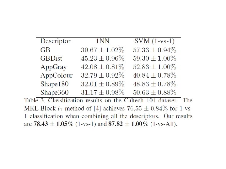
Experimental Results – Caltech 101 1 -NN SVM (1 -vs-1) SVM (1 -vs-All) Shape GB 1 39. 67 1. 02 57. 33 0. 94 62. 98 0. 70 Shape GB 2 45. 23 0. 96 59. 30 1. 00 61. 53 0. 57 Self Similarity 40. 09 0. 98 55. 10 1. 05 60. 83 0. 84 Gist 30. 41 0. 85 45. 56 0. 82 51. 46 0. 79 MKL Block l 1 62. 09 0. 40 72. 05 0. 56 Our 65. 73 0. 77 77. 47 0. 36 Comparisons to the state-of-the-art • Zhang et al. [CVPR 06]: 59. 08 0. 38% by combining shape and texture cues. Frome et al. add colour and get 60. 3 0. 70% [NIPS 2006] and 63. 2% [ICCV 2007]. • Lin et al. [CVPR 07]: 59. 80% by combining 8 features using Kernel Target Alignment • Boiman et al. [CVPR 08]: 72. 8 0. 39% by combining 5 descriptors.

Extending MKL

Extending Our MKL Formulation • Minimisew, b, d ½wtw + i L(f(xi), yi) + l(d) • Subject to constraints on d • where • (xi, yi) is the ith training point. • f(x) = wt d(x) + b • L is a general loss function. • Kd(xi, xj) is a kernel function parameterised by d. • l is a regularizer on the kernel parameters.

Kernel Generalizations • The learnt kernel can now have any functional form as long as • d. K(d) exists and is continuous. • K(d) is strictly positive definite for feasible d. • For example, K(d) = k dk 0 l exp(– dkl 2) • However, not all kernel parameterizations lead to convex formulations. • This does not appear to be a problem for the applications we have tested on.

Regularization Generalizations • Any regulariser can be used as long as it has continuous first derivative with respect to d • We can now put Gaussian rather than Laplacian priors on the kernel weights. • We can have other sparsity promoting priors. • We can, once again, have negative weights.

Loss Function Generalizations • The loss function can be generalized to handle • Regression. • Novelty detection (1 class SVM). • Multi-classification. • Ordinal Regression. • Ranking.

Multiple Kernel Regression Formulation • Minimisew, b, d ½wtw + C i i + l(d) • Subject to • | wt d(xi) + b – yi | + i • i 0 • dk 0 • where • (xi, yi) is the ith training point. • C and are user specified parameters.

Probabilistic Interpretation for Regression • MAP estimation with the following priors and likelihood p(b) = const (improper prior) const e – l(d) if d 0 p(d) = 0 otherwise { p( |d) = p(y|x, , d, b) = |( /2 )Kd|½ e–½ ’K ½(1+ )– 1 e –Max(0, |b – ’K(: , x) – y| – ) is equivalent to the optimization involved in our Multiple Kernel Regression formulation Min , d, b ½ ’Kd + C i Max(0, |b – ’Kd(: , x) – y| – ) + l(d) – ½C log(|Kd|) • This is very similar to the Marginal Likelihood formulation in Gaussian Processes.

Predicting Facial Attractiveness Anandan Chris What is their rating on the milli. Helen scale?

Hot or Not – www. hotornot. com

Regression on Hot or Not Training Data 7. 3 8. 7 6. 5 6. 9 7. 5 6. 5 9. 4 7. 7

Predicting Facial Attractiveness – Features • Geometric features: Face, eyes, nose and lip contours. • Texture patch features: Skin and hair. • HSV colour features: Skin and hair.

Predicting Facial Attractiveness Francis Bach 8. 85 Luc Van Gool Phil Torr 8. 58 8. 38 Richard Hartley 8. 35 Jean Ponce 8. 30

Today – Kernel Combination, Segmentation, and Structured Output • M. Varma and D. Ray, "Learning the discriminative power-invariance trade-off, " in Computer Vision, 2007. ICCV 2007. IEEE 11 th International Conference on, 2007, • Q. Yuan, A. Thangali, V. Ablavsky, and S. Sclaroff, "Multiplicative kernels: Object detection, segmentation and pose estimation, " in Computer Vision and Pattern Recognition, 2008. CVPR 2008 • M. B. Blaschko and C. H. Lampert, "Learning to localize objects with structured output regression, " in ECCV 2008. – but first, Lampert et. al. , CVPR 2008…. • C. Pantofaru, C. Schmid, and M. Hebert, "Object recognition by integrating multiple image segmentations, " CVPR 2008, • Chunhui Gu, Joseph J. Lim, Pablo Arbelaez, Jitendra Malik, Recognition using Regions, CVPR 2009, to appear

Today – Kernel Combination, Segmentation, and Structured Output • M. Varma and D. Ray, "Learning the discriminative power-invariance trade-off, " in Computer Vision, 2007. ICCV 2007. IEEE 11 th International Conference on, 2007, • Q. Yuan, A. Thangali, V. Ablavsky, and S. Sclaroff, "Multiplicative kernels: Object detection, segmentation and pose estimation, " in Computer Vision and Pattern Recognition, 2008. CVPR 2008 • M. B. Blaschko and C. H. Lampert, "Learning to localize objects with structured output regression, " in ECCV 2008. • C. Pantofaru, C. Schmid, and M. Hebert, "Object recognition by integrating multiple image segmentations, " CVPR 2008 • Chunhui Gu, Joseph J. Lim, Pablo Arbelaez, Jitendra Malik, Recognition using Regions, CVPR 2009, to appear

Today – Kernel Combination, Segmentation, and Structured Output • M. Varma and D. Ray, "Learning the discriminative power-invariance trade-off, " in Computer Vision, 2007. ICCV 2007. IEEE 11 th International Conference on, 2007, • Q. Yuan, A. Thangali, V. Ablavsky, and S. Sclaroff, "Multiplicative kernels: Object detection, segmentation and pose estimation, " in Computer Vision and Pattern Recognition, 2008. CVPR 2008 • M. B. Blaschko and C. H. Lampert, "Learning to localize objects with structured output regression, " in ECCV 2008. • C. Pantofaru, C. Schmid, and M. Hebert, "Object recognition by integrating multiple image segmentations, " CVPR 2008 • Chunhui Gu, Joseph J. Lim, Pablo Arbelaez, Jitendra Malik, Recognition using Regions, CVPR 2009, to appear

Recognition using Regions Chunhui Gu, Joseph Lim, Pablo Arbelaez, Jitendra Malik UC Berkeley

Grand Recognition Problem • Detection • Segmentation Tiger • Classification

Region Extraction Region Segmentation Bag of Regions

Region Description g. Pb

Weight Learning • Not all regions are equally important DIK DIJ image J exemplar I DIJ = Σi wi · di. J image K and di. J=minj χ2(fi. I, fj. J) want: DIK > DIJ Max-margin formulation results in a sparse solution of weights. 1. Frome et al. NIPS ‘ 06

Weight Learning

Detection/Segmentation Algorithm Exemplars Detection Images Verification classifier Ground truths Region matching based voting Query Constrained segmenter Initial Hypotheses Segmentation

Voting Exemplar Query

Verification • For exemplar 1, 2, …, N of class C, define likelihood function of query image J: where f converts a distance to a similarity measure (e. g. logistic regression, negation) • The predicted category label for image J:

Segmentation Query Initial Seeds Exemplar Constrained Mask Result

Results

ETHZ Shape (Ferrari et al. 06) • Contains 255 images of 5 diverse shape‐based classes.

Detection/Segmentation Results • Significantly outperforms the state of the art (Ferrari et al. CVPR 07) – 87. 1% vs. 67. 2% det. rate at 0. 3 FFPI • 75. 7% Average Precision rate in segmentation, >20% boost w. r. t. bounding boxes

A Comparison to Sliding Window

Caltech 101 (Fei‐Fei et al. 04) • 102 classes, 31‐ 800 images/class

Classification Rate in Caltech 101

Results with Cue Combination

Conclusion • Introduce a unified framework for object detection, segmentation and classification • Regions encode shape and scale information of objects naturally • Cue combination improves recognition performance • Region‐based Hough voting significantly reduces number of candidate windows for detection

Thank You

Multiplicative kernels for parameterized detectors Object Detection (binary classification) Umm, this doesn’t look like a hand A hand is here! Foreground State Estimation features Inference Angles between fingers, view angle. . . Learning a Family of Detectors, Yuan /Sclaroff CVPR 2008

Proposed Approach We try to learn a function which tells whether is an instance of the object with foreground state. Learning a Family of Detectors, Yuan /Sclaroff CVPR 2008

Why If we fix , - intuitions is a detector of a specific Parameter estimation can be achieved by searching of best via. Learning a Family of Detectors, Yuan /Sclaroff CVPR 2008

Learning of function C Assume C can be factorized into a feature space mapping and a weight vector : where Learning a Family of Detectors, Yuan /Sclaroff CVPR 2008

Approximation of W is approximated by basis function expansion: where vectors are unknowns and Learning a Family of Detectors, Yuan /Sclaroff CVPR 2008

Kernel Representation If we plug and The unknowns are in . into is the data term. Learning a Family of Detectors, Yuan /Sclaroff CVPR 2008

Kernel Representation If we solve the binary classification problem by SVM, the actual kernel is, where Learning a Family of Detectors, Yuan /Sclaroff CVPR 2008

Kernel Representation After SVM learning, the classification function becomes where is the weight of i-th support vector and Learning a Family of Detectors, Yuan /Sclaroff CVPR 2008

Short Summary We have a way to learn evaluates tuples. which corresponds to a family of detectors tuned to different. Feature sharing is implicit via sharing of support vectors. Learning a Family of Detectors, Yuan /Sclaroff CVPR 2008

Training Process Each training sample is in the form of a tuple x 1 = , . =0 x 2 = , = 30 x 3 = , = 70 Foreground tuples x= , = 0, 10, 20, … For a background tuple, the parameter can be random. We propose an iterative bootstrap training process to avoid potentially huge number of background training tuples. Learning a Family of Detectors, Yuan /Sclaroff CVPR 2008

Feasibility Experiment III Vehicle data set, 12 view categories. Learning a Family of Detectors, Yuan /Sclaroff CVPR 2008

Feasibility Experiment III is an RBF kernel defined with Euclidean distance in HOG space kernel. is a linear kernel. Detection accuracy compared with previous detection methods. Learning a Family of Detectors, Yuan /Sclaroff CVPR 2008

Feasibility Experiment III Vehicle view angle estimation (multi-classification) Baseline method (12 subclass detectors): 62. 4% Torralba et al. 2004: 65. 0% In both methods, view labels of all FG training samples are given (1405 in total). Multiplicative Kernels: # view labels needed in our approach #modes accuracy 400 65. 6% 68. 0% 800 71. 7%

Next Lecture – Image Context • A. Torralba, K. P. Murphy, and W. T. Freeman, "Contextual models for object detection using boosted random fields, " in Advances in Neural Information Processing Systems 17 (NIPS), 2005. • D. Hoiem, A. A. Efros, and M. Hebert, "Putting objects in perspective, " in Computer Vision and Pattern Recognition, 2006 • L. -J. Li and L. Fei-Fei, "What, where and who? classifying events by scene and object recognition, " in Computer Vision, 2007. • G. Heitz and D. Koller, "Learning spatial context: Using stuff to find things, " in ECCV 2008, pp. 30 -43. • S. Gould, J. Arfvidsson, A. Kaehler, B. Sapp, M. Messner, G. R. Bradski, P. Baumstarck, S. Chung, A. Y. Ng: Peripheral-Foveal Vision for Real-time Object Recognition and Tracking in Video. IJCAI 2007 • Y. Li and R. Nevatia, "Key object driven multi-category object recognition, localization and tracking using spatio-temporal context, " in ECCV 2008