CS 2770 Computer Vision Local Feature Detection and

CS 2770: Computer Vision Local Feature Detection and Description Prof. Adriana Kovashka University of Pittsburgh February 9, 2017

Plan for today • Feature detection / keypoint extraction – Corner detection – Blob detection • Feature description (of detected features)

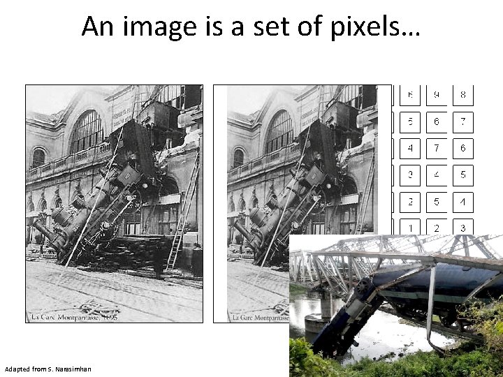
An image is a set of pixels… What we see Adapted from S. Narasimhan What a computer sees Source: S. Narasimhan

Problems with pixel representation • Not invariant to small changes – Translation – Illumination – etc. • Some parts of an image are more important than others • What do we want to represent?

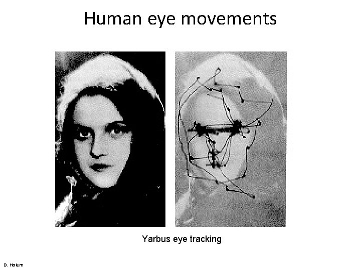
Human eye movements Yarbus eye tracking D. Hoiem

Local features • Local means that they only cover a small part of the image • There will be many local features detected in an image • Later we’ll talk about how to use those to compute a representation of the whole image • Local features usually exploit image gradients, ignore color

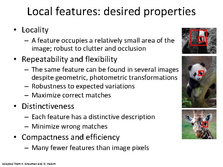
Local features: desired properties • Locality – A feature occupies a relatively small area of the image; robust to clutter and occlusion • Repeatability and flexibility – The same feature can be found in several images despite geometric, photometric transformations – Robustness to expected variations – Maximize correct matches • Distinctiveness – Each feature has a distinctive description – Minimize wrong matches • Compactness and efficiency – Many fewer features than image pixels Adapted from K. Grauman and D. Hoiem

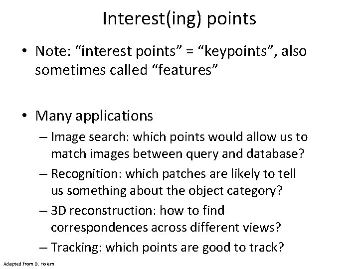
Interest(ing) points • Note: “interest points” = “keypoints”, also sometimes called “features” • Many applications – Image search: which points would allow us to match images between query and database? – Recognition: which patches are likely to tell us something about the object category? – 3 D reconstruction: how to find correspondences across different views? – Tracking: which points are good to track? Adapted from D. Hoiem

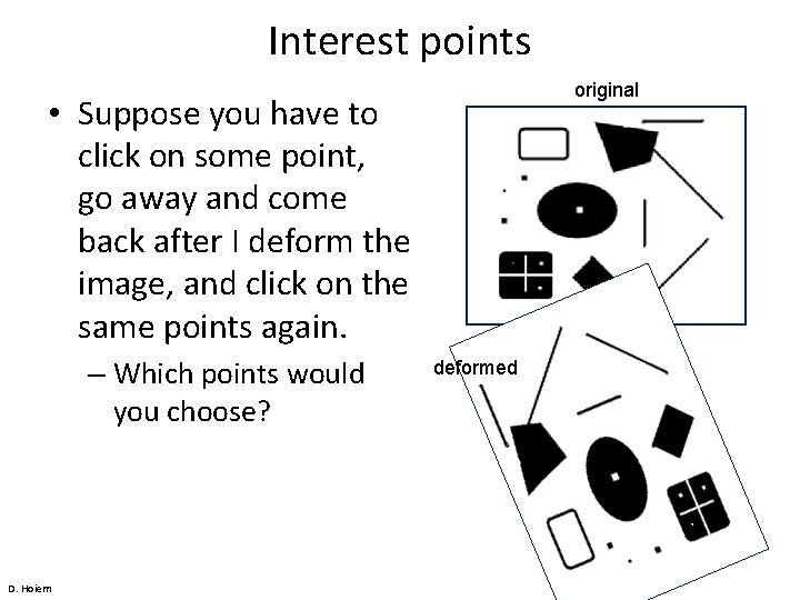
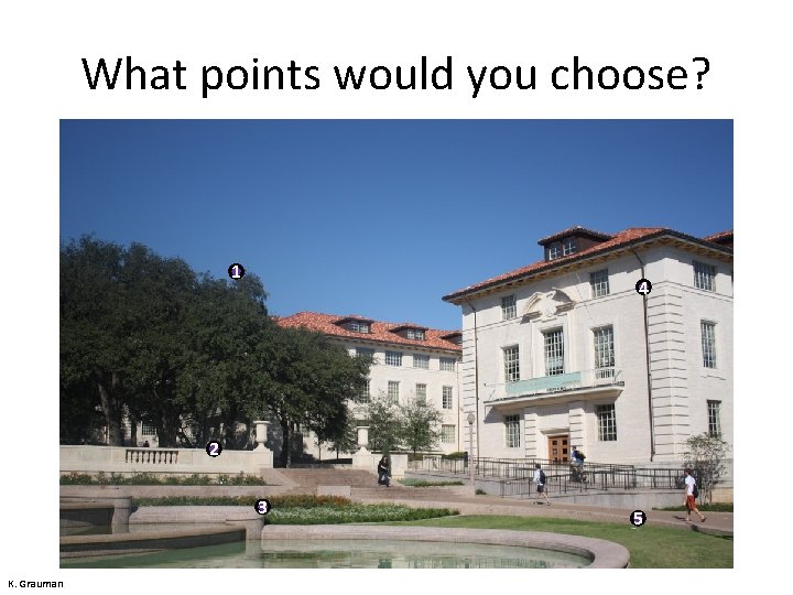
Interest points original • Suppose you have to click on some point, go away and come back after I deform the image, and click on the same points again. – Which points would you choose? D. Hoiem deformed

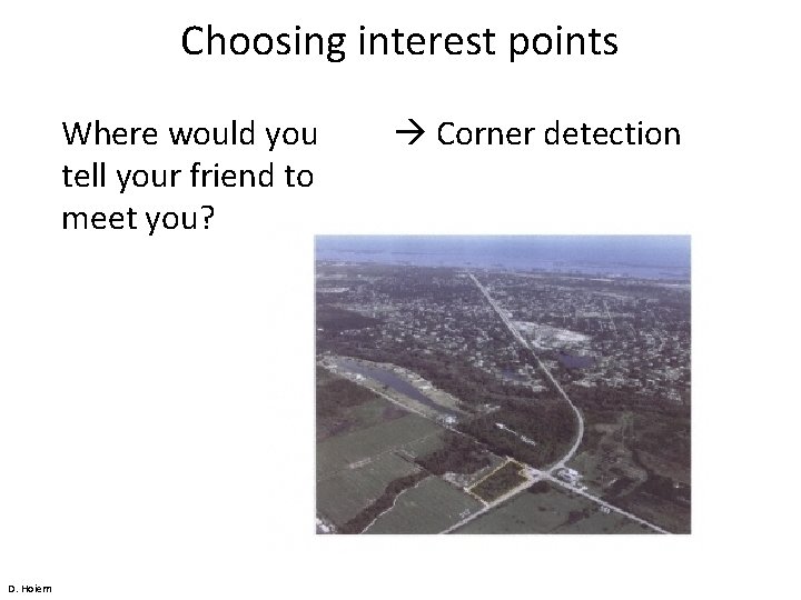
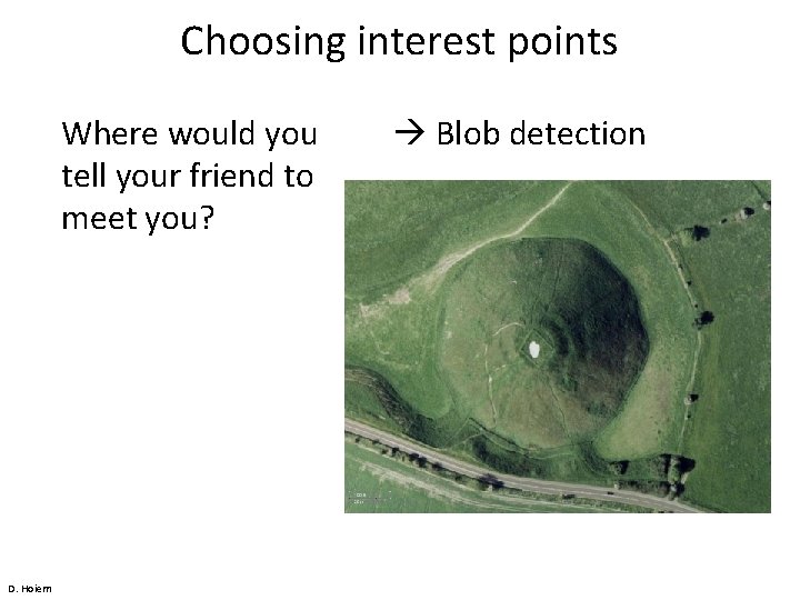
Choosing interest points Where would you tell your friend to meet you? D. Hoiem Corner detection

Choosing interest points Where would you tell your friend to meet you? D. Hoiem Blob detection

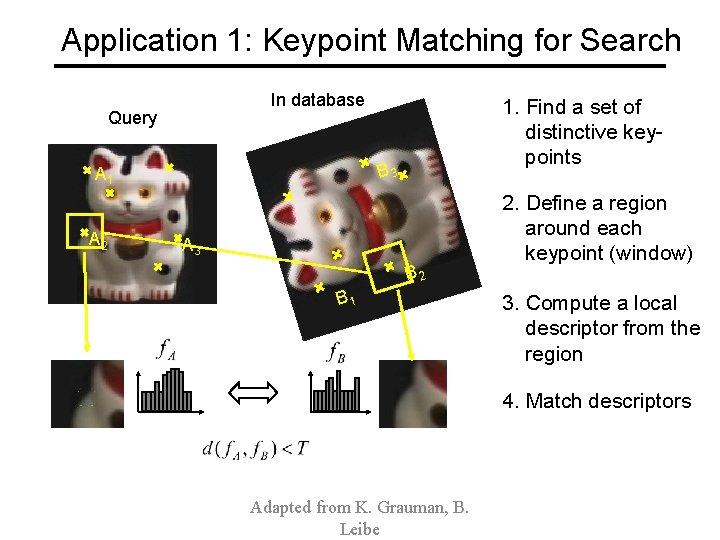
Application 1: Keypoint Matching for Search In database Query B 3 A 1 A 2 1. Find a set of distinctive keypoints A 3 B 2 B 1 2. Define a region around each keypoint (window) 3. Compute a local descriptor from the region 4. Match descriptors Adapted from K. Grauman, B. Leibe

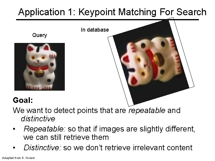
Application 1: Keypoint Matching For Search Query In database Goal: We want to detect points that are repeatable and distinctive • Repeatable: so that if images are slightly different, we can still retrieve them • Distinctive: so we don’t retrieve irrelevant content Adapted from D. Hoiem

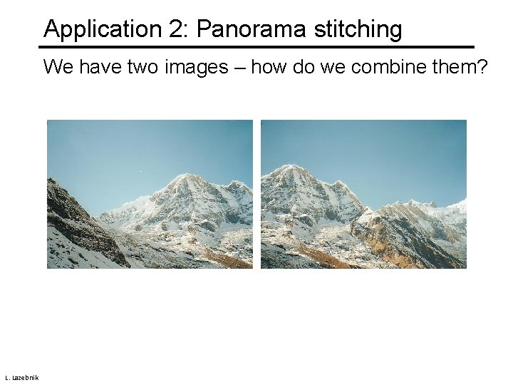
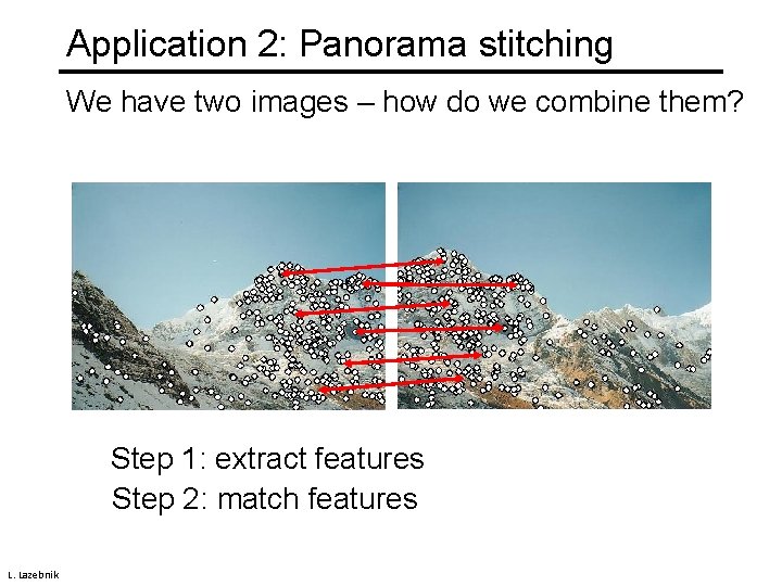
Application 2: Panorama stitching We have two images – how do we combine them? L. Lazebnik

Application 2: Panorama stitching We have two images – how do we combine them? Step 1: extract features Step 2: match features L. Lazebnik

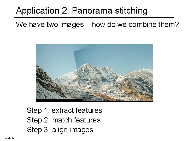
Application 2: Panorama stitching We have two images – how do we combine them? Step 1: extract features Step 2: match features Step 3: align images L. Lazebnik

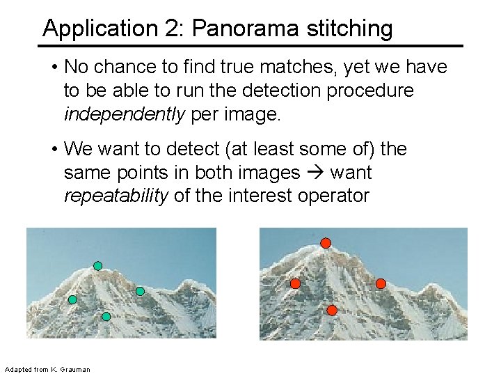
Application 2: Panorama stitching • No chance to find true matches, yet we have to be able to run the detection procedure independently per image. • We want to detect (at least some of) the same points in both images want repeatability of the interest operator Adapted from K. Grauman

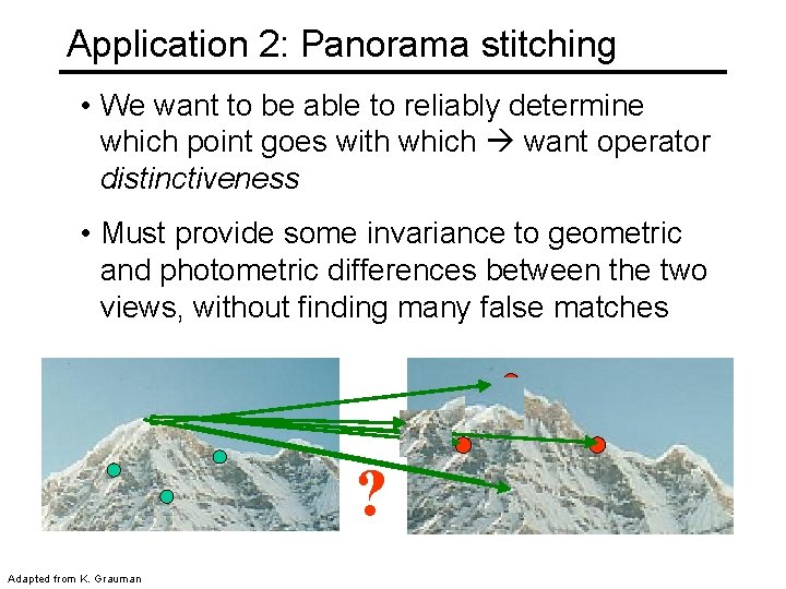
Application 2: Panorama stitching • We want to be able to reliably determine which point goes with which want operator distinctiveness • Must provide some invariance to geometric and photometric differences between the two views, without finding many false matches ? Adapted from K. Grauman

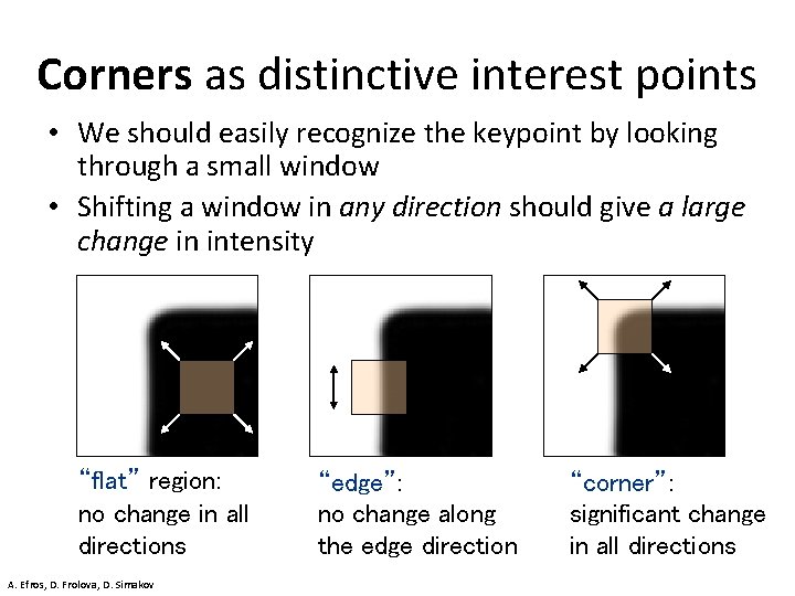
Corners as distinctive interest points • We should easily recognize the keypoint by looking through a small window • Shifting a window in any direction should give a large change in intensity “flat” region: no change in all directions A. Efros, D. Frolova, D. Simakov “edge”: no change along the edge direction “corner”: significant change in all directions

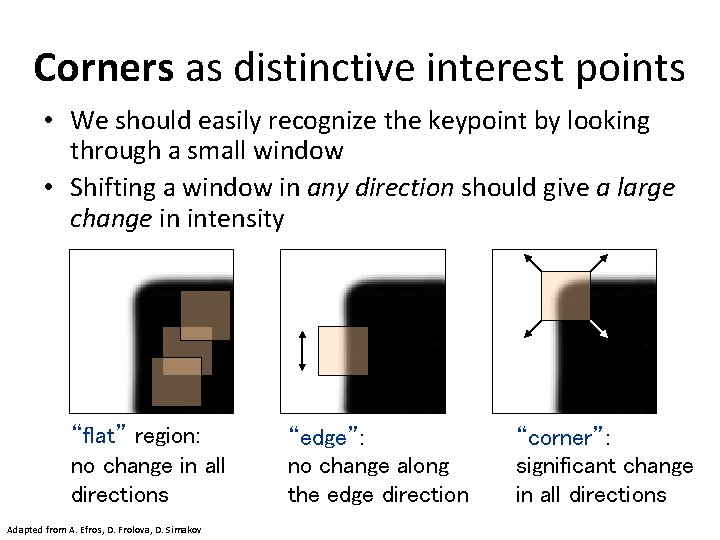
Corners as distinctive interest points • We should easily recognize the keypoint by looking through a small window • Shifting a window in any direction should give a large change in intensity “flat” region: no change in all directions Adapted from A. Efros, D. Frolova, D. Simakov “edge”: no change along the edge direction “corner”: significant change in all directions

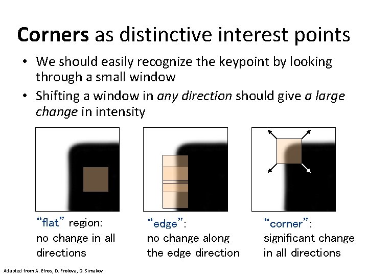
Corners as distinctive interest points • We should easily recognize the keypoint by looking through a small window • Shifting a window in any direction should give a large change in intensity “flat” region: no change in all directions Adapted from A. Efros, D. Frolova, D. Simakov “edge”: no change along the edge direction “corner”: significant change in all directions

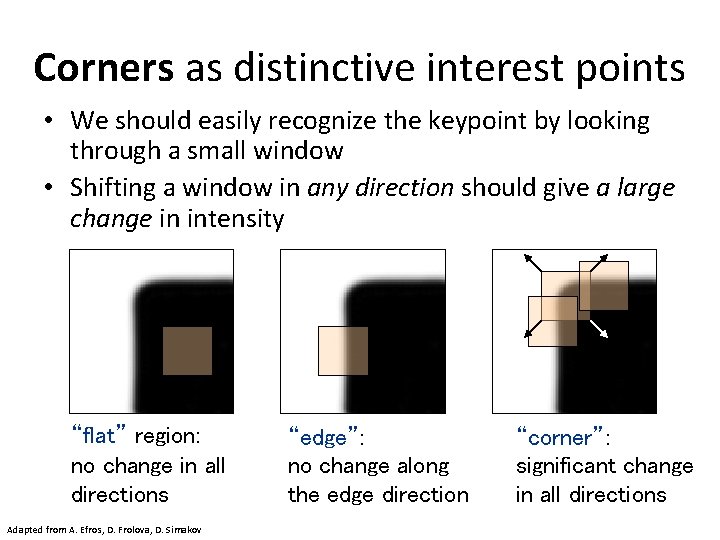
Corners as distinctive interest points • We should easily recognize the keypoint by looking through a small window • Shifting a window in any direction should give a large change in intensity “flat” region: no change in all directions Adapted from A. Efros, D. Frolova, D. Simakov “edge”: no change along the edge direction “corner”: significant change in all directions

Corners as distinctive interest points • We should easily recognize the keypoint by looking through a small window • Shifting a window in any direction should give a large change in intensity “flat” region: no change in all directions Adapted from A. Efros, D. Frolova, D. Simakov “edge”: no change along the edge direction “corner”: significant change in all directions

What points would you choose? 1 4 2 3 K. Grauman 5

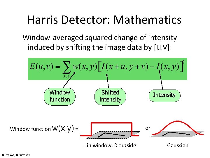
Harris Detector: Mathematics Window-averaged squared change of intensity induced by shifting the image data by [u, v]: Window function Shifted intensity Window function w(x, y) = or 1 in window, 0 outside D. Frolova, D. Simakov Intensity Gaussian

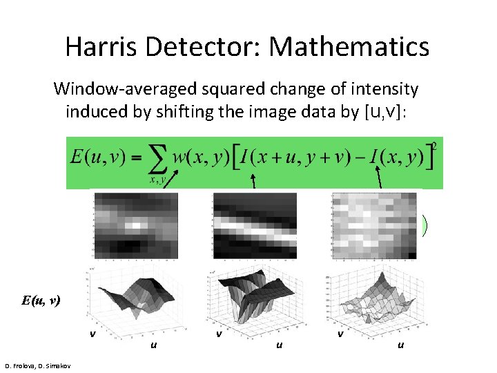
Harris Detector: Mathematics Window-averaged squared change of intensity induced by shifting the image data by [u, v]: Window function Shifted intensity Intensity E(u, v) v D. Frolova, D. Simakov u v u

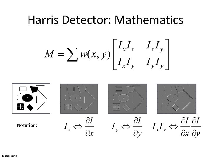
Harris Detector: Mathematics Notation: K. Grauman

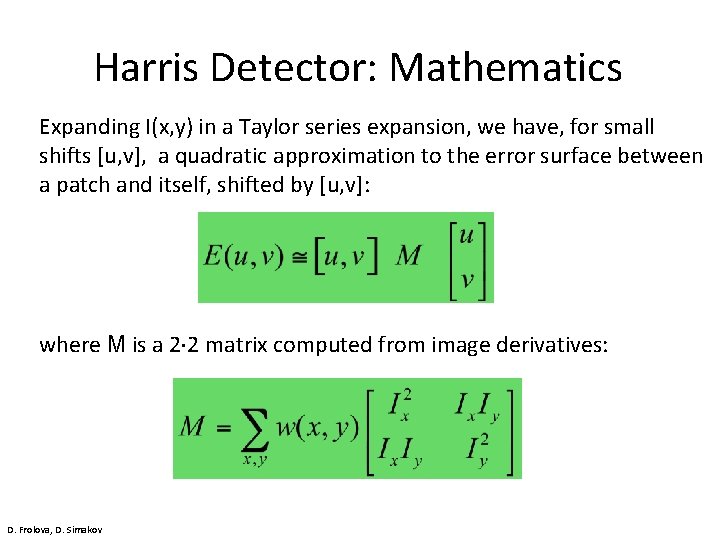
Harris Detector: Mathematics Expanding I(x, y) in a Taylor series expansion, we have, for small shifts [u, v], a quadratic approximation to the error surface between a patch and itself, shifted by [u, v]: where M is a 2× 2 matrix computed from image derivatives: D. Frolova, D. Simakov

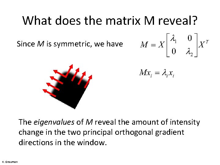
What does the matrix M reveal? Since M is symmetric, we have The eigenvalues of M reveal the amount of intensity change in the two principal orthogonal gradient directions in the window. K. Grauman

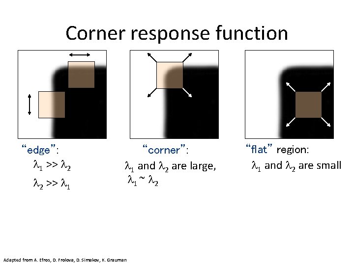
Corner response function “edge”: 1 >> 2 2 >> 1 “corner”: 1 and 2 are large, 1 ~ 2 Adapted from A. Efros, D. Frolova, D. Simakov, K. Grauman “flat” region: 1 and 2 are small

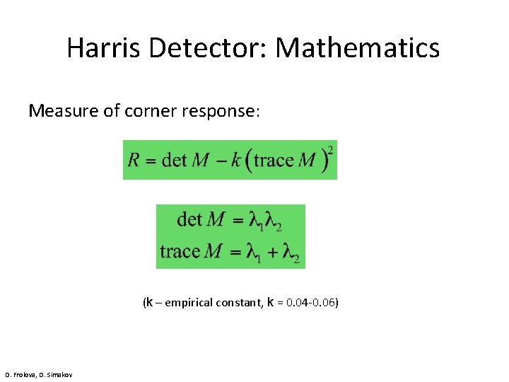
Harris Detector: Mathematics Measure of corner response: (k – empirical constant, k = 0. 04 -0. 06) D. Frolova, D. Simakov

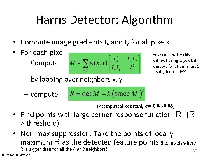
Harris Detector: Algorithm • Compute image gradients Ix and Iy for all pixels • For each pixel How can I write this without using w(x, y), if – Compute window function is just 1 by looping over neighbors x, y inside, 0 outside? – compute (k : empirical constant, k = 0. 04 -0. 06) • Find points with large corner response function R (R > threshold) • Non-max suppression: Take the points of locally maximum R as the detected feature points (i. e. , pixels where R is bigger than for all the 4 or 8 neighbors) D. Frolova, D. Simakov 32

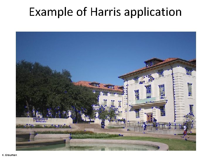
Example of Harris application K. Grauman

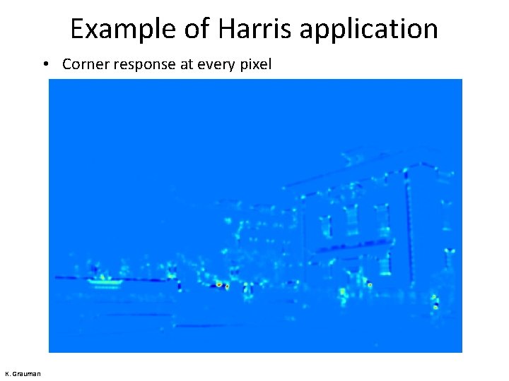
Example of Harris application • Corner response at every pixel K. Grauman

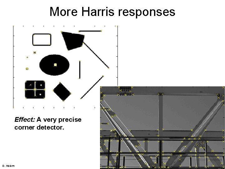
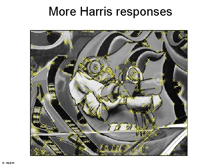
More Harris responses Effect: A very precise corner detector. D. Hoiem

More Harris responses D. Hoiem

Properties: Invariance vs covariance “A function is invariant under a certain family of transformations if its value does not change when a transformation from this family is applied to its argument. A function is covariant when it commutes with the transformation, i. e. , applying the transformation to the argument of the function has the same effect as applying the transformation to the output of the function. […] [For example, ] the area of a 2 D surface is invariant under 2 D rotations, since rotating a 2 D surface does not make it any smaller or bigger. But the orientation of the major axis of inertia of the surface is covariant under the same family of transformations, since rotating a 2 D surface will affect the orientation of its major axis in exactly the same way. ” “Local Invariant Feature Detectors: A Survey” by Tinne Tuytelaars and Krystian Mikolajczyk, in Foundations and Trends in Computer Graphics and Vision Vol. 3, No. 3 (2007) 177– 280 Chapter 1, 3. 2, 7 http: //homes. esat. kuleuven. be/%7 Etuytelaa/FT_survey_interestpoints 08. pdf

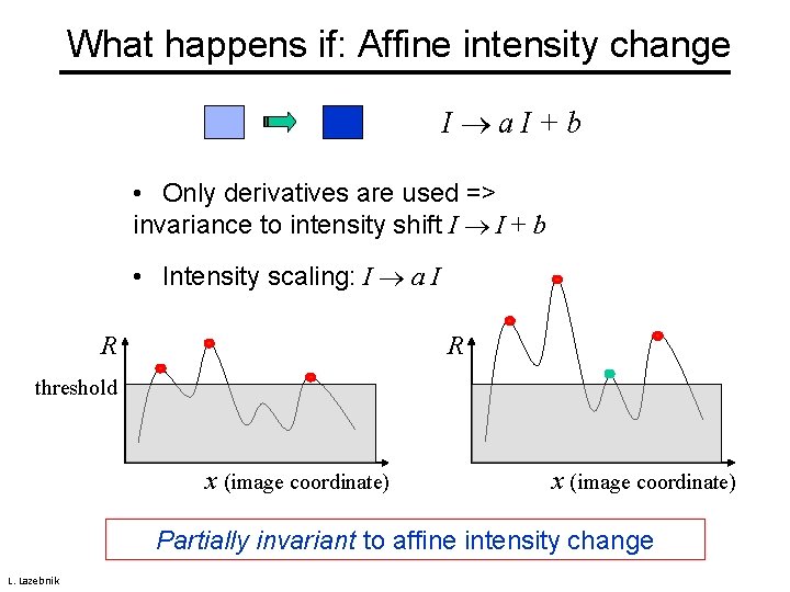
What happens if: Affine intensity change I a. I+b • Only derivatives are used => invariance to intensity shift I I + b • Intensity scaling: I a I R R threshold x (image coordinate) Partially invariant to affine intensity change L. Lazebnik

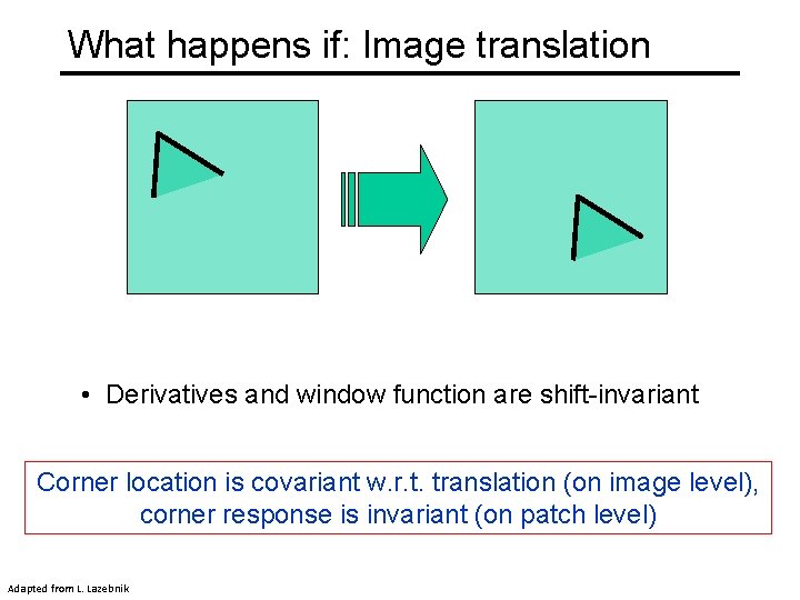
What happens if: Image translation • Derivatives and window function are shift-invariant Corner location is covariant w. r. t. translation (on image level), corner response is invariant (on patch level) Adapted from L. Lazebnik

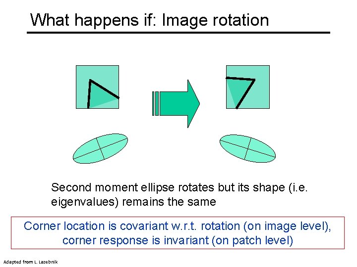
What happens if: Image rotation Second moment ellipse rotates but its shape (i. e. eigenvalues) remains the same Corner location is covariant w. r. t. rotation (on image level), corner response is invariant (on patch level) Adapted from L. Lazebnik

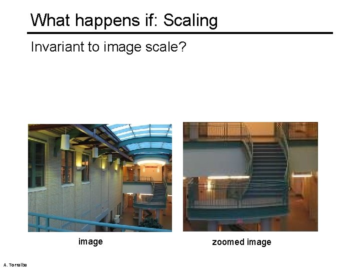
What happens if: Scaling Invariant to image scale? image A. Torralba zoomed image

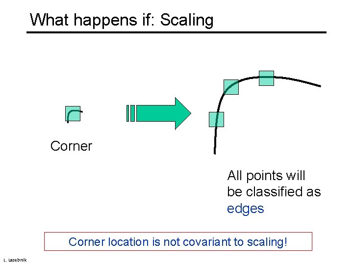
What happens if: Scaling Corner All points will be classified as edges Corner location is not covariant to scaling! L. Lazebnik

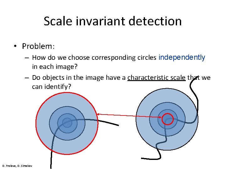
Scale invariant detection • Problem: – How do we choose corresponding circles independently in each image? – Do objects in the image have a characteristic scale that we can identify? D. Frolova, D. Simakov

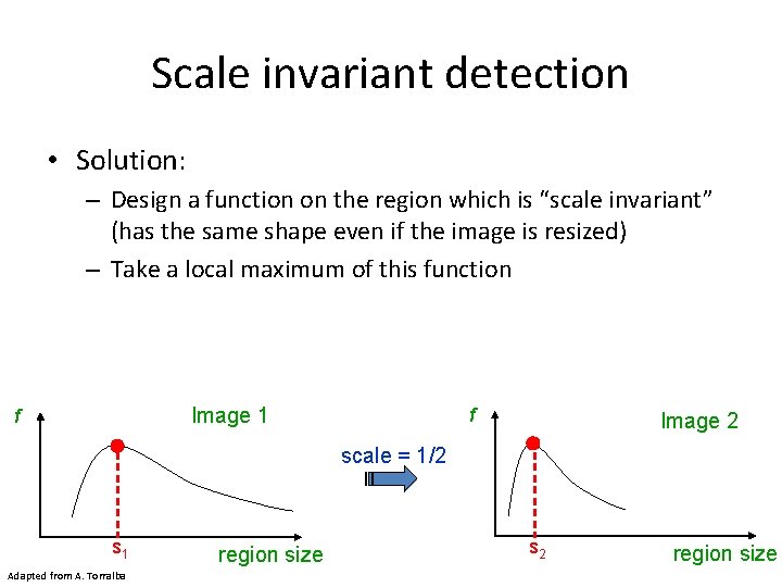
Scale invariant detection • Solution: – Design a function on the region which is “scale invariant” (has the same shape even if the image is resized) – Take a local maximum of this function Image 1 f f Image 2 scale = 1/2 s 1 Adapted from A. Torralba region size s 2 region size

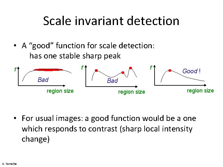
Scale invariant detection • A “good” function for scale detection: has one stable sharp peak f f Bad region size f Good ! Bad region size • For usual images: a good function would be a one which responds to contrast (sharp local intensity change) A. Torralba

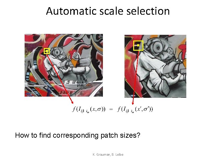
Automatic scale selection How to find corresponding patch sizes? K. Grauman, B. Leibe

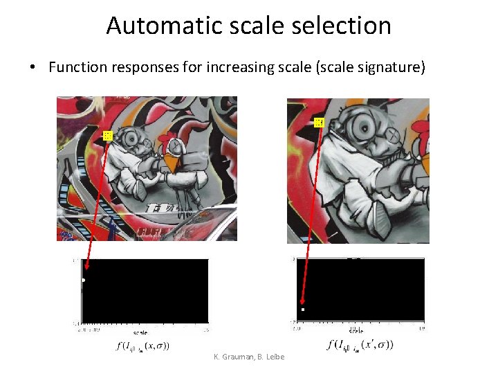
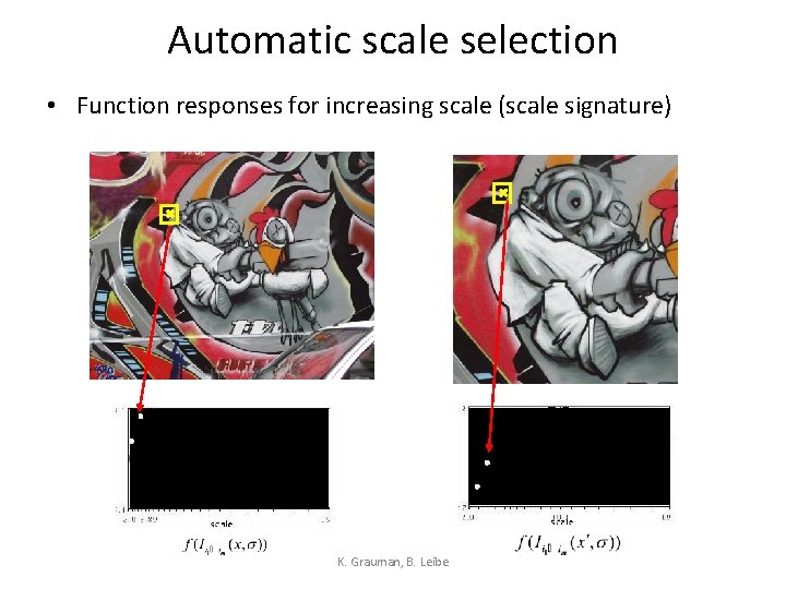
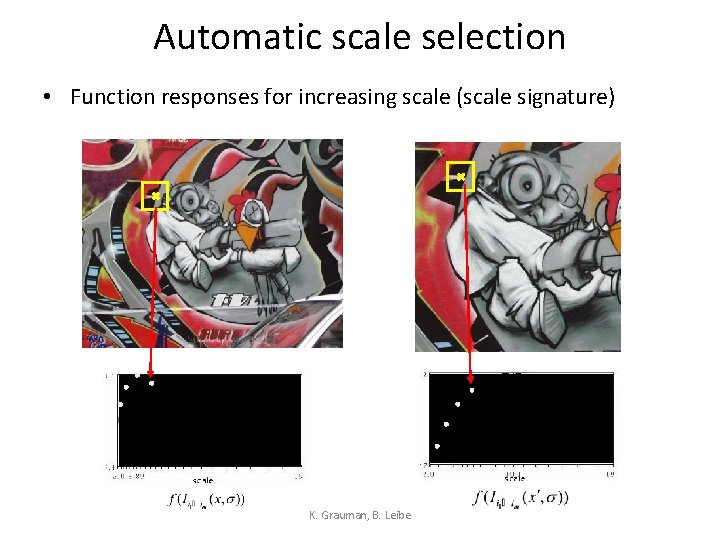
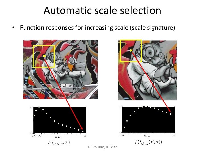
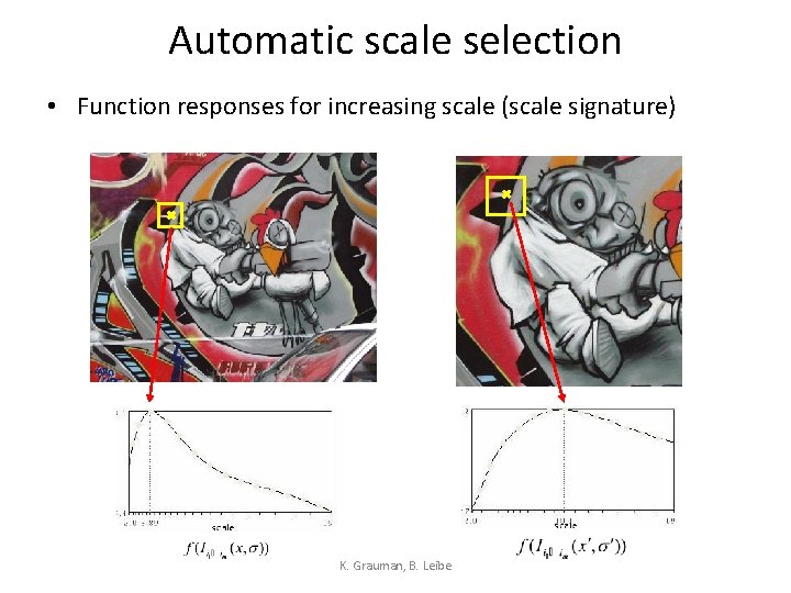
Automatic scale selection • Function responses for increasing scale (scale signature) K. Grauman, B. Leibe

Automatic scale selection • Function responses for increasing scale (scale signature) K. Grauman, B. Leibe

Automatic scale selection • Function responses for increasing scale (scale signature) K. Grauman, B. Leibe

Automatic scale selection • Function responses for increasing scale (scale signature) K. Grauman, B. Leibe

Automatic scale selection • Function responses for increasing scale (scale signature) K. Grauman, B. Leibe

Automatic scale selection • Function responses for increasing scale (scale signature) K. Grauman, B. Leibe

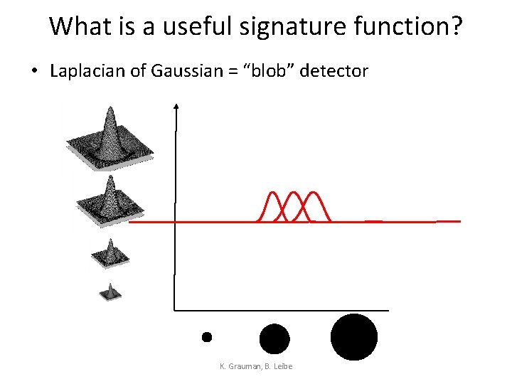
What is a useful signature function? • Laplacian of Gaussian = “blob” detector K. Grauman, B. Leibe

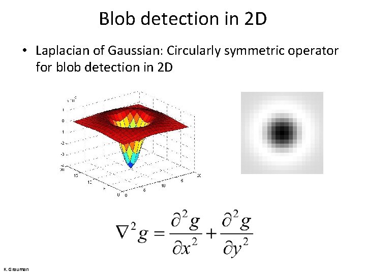
Blob detection in 2 D • Laplacian of Gaussian: Circularly symmetric operator for blob detection in 2 D K. Grauman

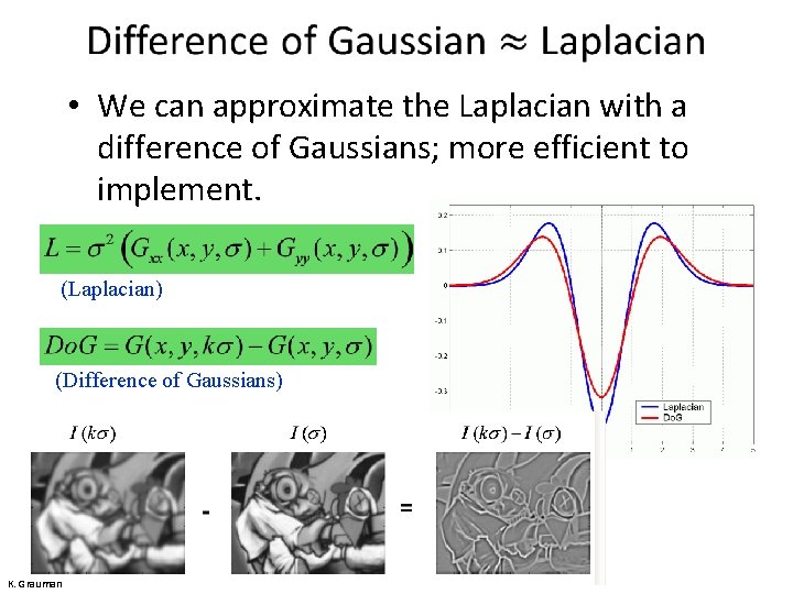
• We can approximate the Laplacian with a difference of Gaussians; more efficient to implement. (Laplacian) (Difference of Gaussians) K. Grauman

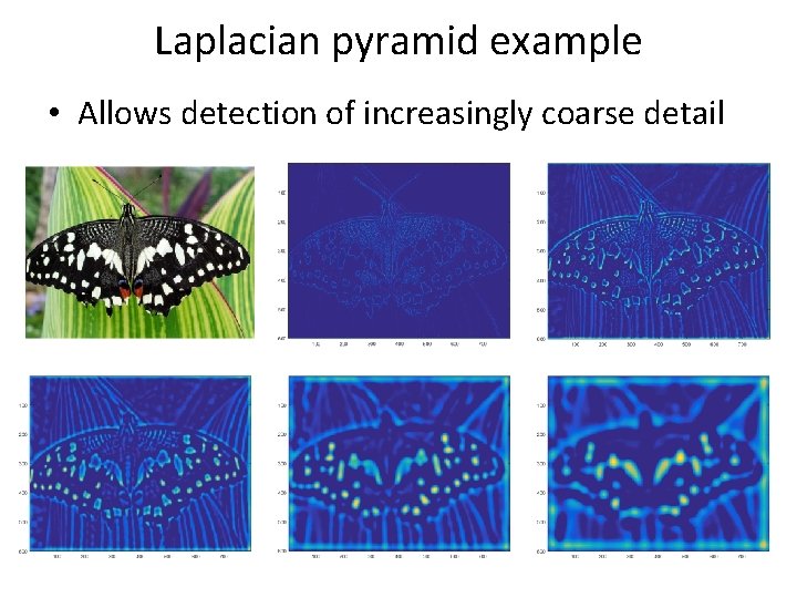
Laplacian pyramid example • Allows detection of increasingly coarse detail

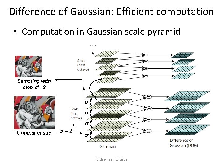
Difference of Gaussian: Efficient computation • Computation in Gaussian scale pyramid Sampling with step s 4 =2 s s s Original image s K. Grauman, B. Leibe

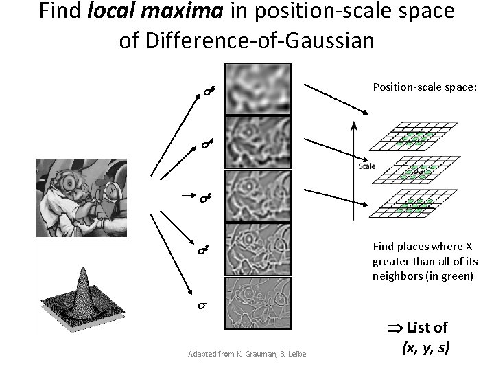
Find local maxima in position-scale space of Difference-of-Gaussian s 5 Position-scale space: s 4 s 3 s 2 Find places where X greater than all of its neighbors (in green) s Adapted from K. Grauman, B. Leibe List of (x, y, s)

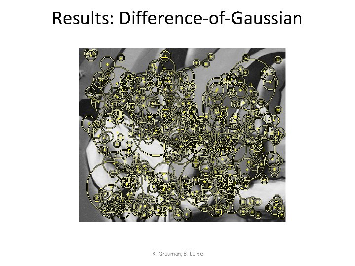
Results: Difference-of-Gaussian K. Grauman, B. Leibe

Plan for today • Feature detection / keypoint extraction – Corner detection – Blob detection • Feature description (of detected features)

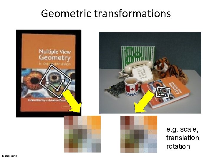
Geometric transformations e. g. scale, translation, rotation K. Grauman

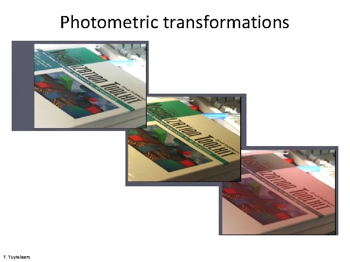
Photometric transformations T. Tuytelaars

Scale-Invariant Feature Transform (SIFT) descriptor [Lowe, ICCV 1999] Histogram of oriented gradients • Captures important texture information • Robust to small translations / affine deformations K. Grauman, B. Leibe

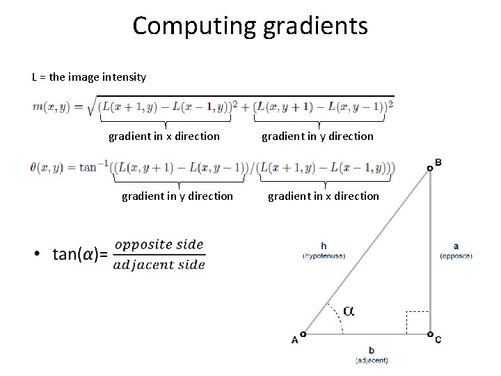
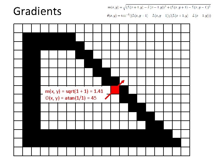
Computing gradients L = the image intensity gradient in x direction gradient in y direction • gradient in y direction gradient in x direction

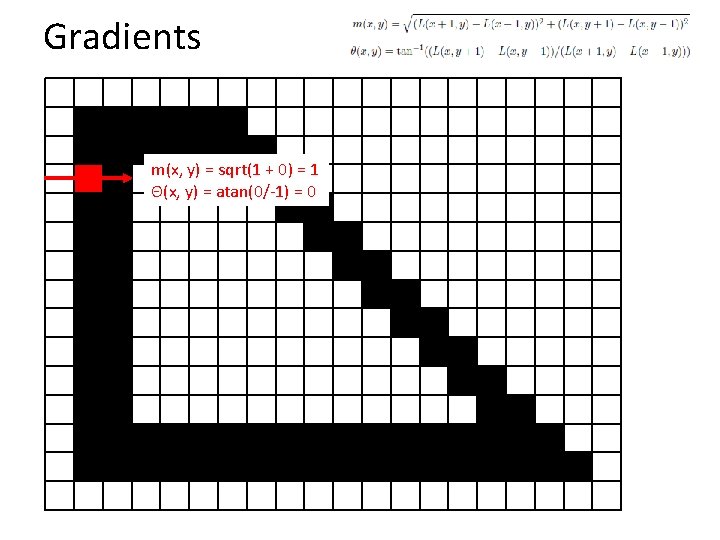
Gradients m(x, y) = sqrt(1 + 0) = 1 Θ(x, y) = atan(0/-1) = 0

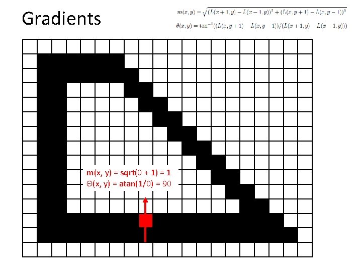
Gradients m(x, y) = sqrt(0 + 1) = 1 Θ(x, y) = atan(1/0) = 90

Gradients m(x, y) = sqrt(1 + 1) = 1. 41 Θ(x, y) = atan(1/1) = 45

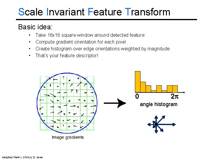
Scale Invariant Feature Transform Basic idea: • • Take 16 x 16 square window around detected feature Compute gradient orientation for each pixel Create histogram over edge orientations weighted by magnitude That’s your feature descriptor! 0 2 angle histogram Adapted from L. Zitnick, D. Lowe

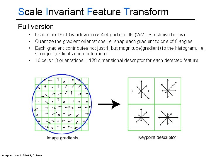
Scale Invariant Feature Transform Full version • • Divide the 16 x 16 window into a 4 x 4 grid of cells (2 x 2 case shown below) Quantize the gradient orientations i. e. snap each gradient to one of 8 angles Each gradient contributes not just 1, but magnitude(gradient) to the histogram, i. e. stronger gradients contribute more 16 cells * 8 orientations = 128 dimensional descriptor for each detected feature Adapted from L. Zitnick, D. Lowe

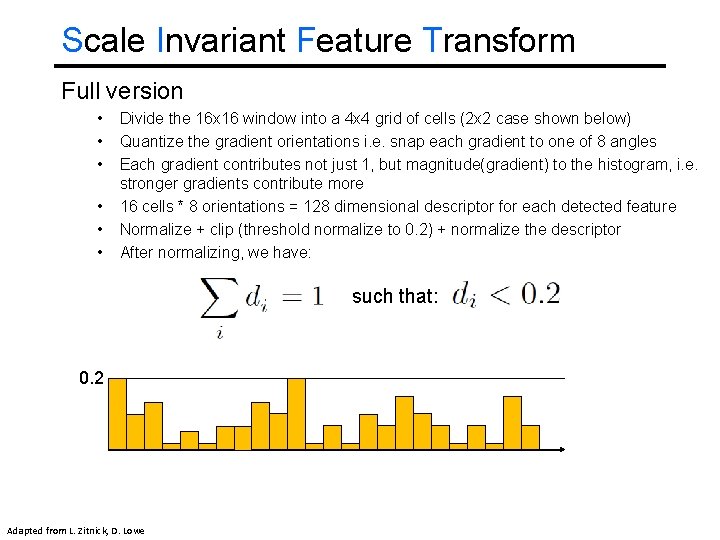
Scale Invariant Feature Transform Full version • • • Divide the 16 x 16 window into a 4 x 4 grid of cells (2 x 2 case shown below) Quantize the gradient orientations i. e. snap each gradient to one of 8 angles Each gradient contributes not just 1, but magnitude(gradient) to the histogram, i. e. stronger gradients contribute more 16 cells * 8 orientations = 128 dimensional descriptor for each detected feature Normalize + clip (threshold normalize to 0. 2) + normalize the descriptor After normalizing, we have: such that: 0. 2 Adapted from L. Zitnick, D. Lowe

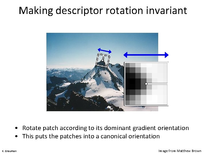
Making descriptor rotation invariant CSE 576: Computer Vision • Rotate patch according to its dominant gradient orientation • This puts the patches into a canonical orientation K. Grauman Image from Matthew Brown

SIFT is robust • Can handle changes in viewpoint • Up to about 60 degree out of plane rotation • Can handle significant changes in illumination • Sometimes even day vs. night (below) • Fast and efficient—can run in real time • Can be made to work without feature detection, resulting in “dense SIFT” (more points means robustness to occlusion) • One commonly used implementation • http: //www. vlfeat. org/overview/sift. html Adapted from S. Seitz

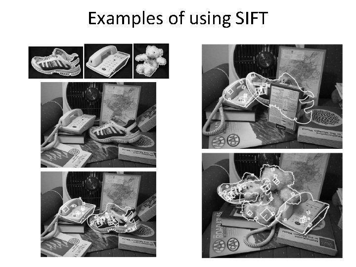
Examples of using SIFT

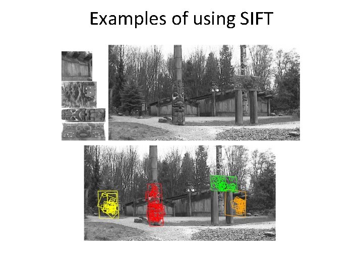
Examples of using SIFT

Examples of using SIFT Images from S. Seitz

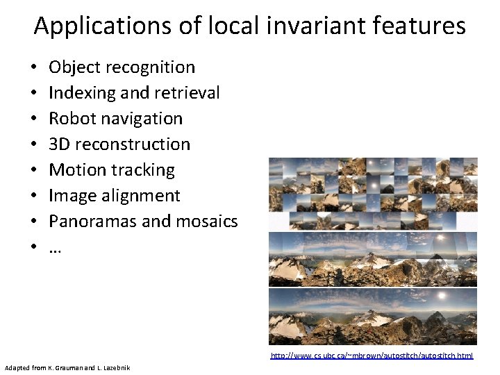
Applications of local invariant features • • Object recognition Indexing and retrieval Robot navigation 3 D reconstruction Motion tracking Image alignment Panoramas and mosaics … http: //www. cs. ubc. ca/~mbrown/autostitch. html Adapted from K. Grauman and L. Lazebnik

Additional references • Survey paper on local features – “Local Invariant Feature Detectors: A Survey” by Tinne Tuytelaars and Krystian Mikolajczyk, in Foundations and Trends in Computer Graphics and Vision Vol. 3, No. 3 (2007) 177– 280 (mostly Chapters 1, 3. 2, 7) http: //homes. esat. kuleuven. be/%7 Etuytelaa/FT_survey_interestpoint s 08. pdf • Making Harris detection scale-invariant – “Indexing based on scale invariant interest points” by Krystian Mikolajczyk and Cordelia Schmid, in ICCV 2001 https: //hal. archivesouvertes. fr/file/index/docid/548276/filename/mikolajc. ICCV 2001. pdf • SIFT paper by David Lowe – “Distinctive Image Features from Scale-Invariant Keypoints” by David G. Lowe, in IJCV 2004 http: //www. cs. ubc. ca/~lowe/papers/ijcv 04. pdf

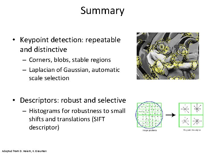
Summary • Keypoint detection: repeatable and distinctive – Corners, blobs, stable regions – Laplacian of Gaussian, automatic scale selection • Descriptors: robust and selective – Histograms for robustness to small shifts and translations (SIFT descriptor) Adapted from D. Hoiem, K. Grauman