CS 267 Applications of Parallel Computers Unstructured Multigrid

CS 267: Applications of Parallel Computers Unstructured Multigrid for Linear Systems James Demmel (based in part on material from Mark Adams) www. cs. berkeley. edu/~demmel/cs 267_Spr 05

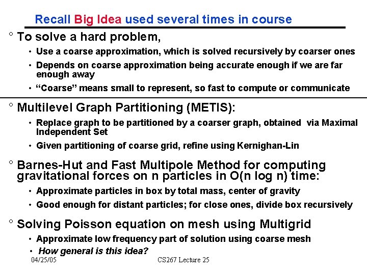
Recall Big Idea used several times in course ° To solve a hard problem, • Use a coarse approximation, which is solved recursively by coarser ones • Depends on coarse approximation being accurate enough if we are far enough away • “Coarse” means small to represent, so fast to compute or communicate ° Multilevel Graph Partitioning (METIS): • Replace graph to be partitioned by a coarser graph, obtained via Maximal Independent Set • Given partitioning of coarse grid, refine using Kernighan-Lin ° Barnes-Hut and Fast Multipole Method for computing gravitational forces on n particles in O(n log n) time: • Approximate particles in box by total mass, center of gravity • Good enough for distant particles; for close ones, divide box recursively ° Solving Poisson equation on mesh using Multigrid • Approximate low frequency part of solution using coarse mesh • How general is this idea? 04/25/05 CS 267 Lecture 25

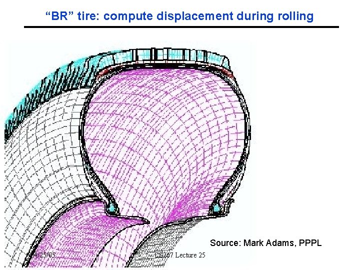
“BR” tire: compute displacement during rolling Source: Mark Adams, PPPL 04/25/05 CS 267 Lecture 25

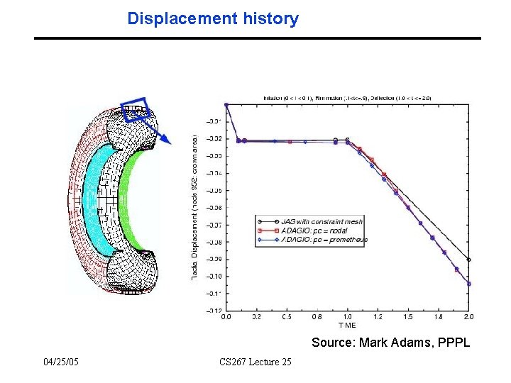
Displacement history Source: Mark Adams, PPPL 04/25/05 CS 267 Lecture 25

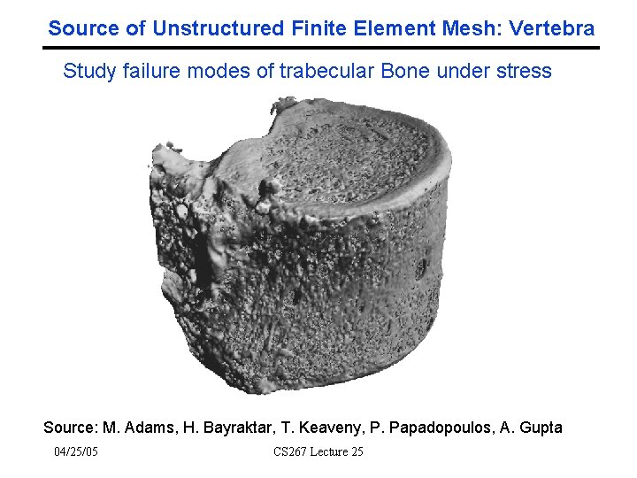
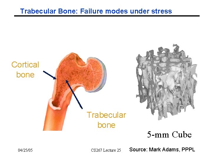
Source of Unstructured Finite Element Mesh: Vertebra Study failure modes of trabecular Bone under stress Source: M. Adams, H. Bayraktar, T. Keaveny, P. Papadopoulos, A. Gupta 04/25/05 CS 267 Lecture 25

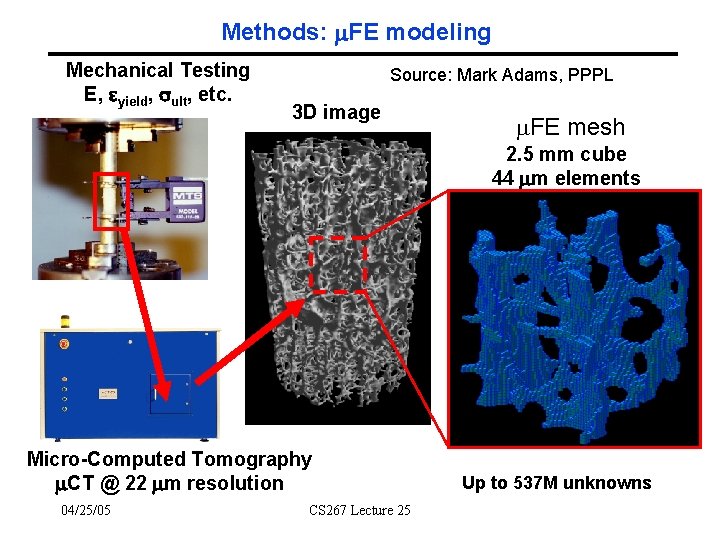
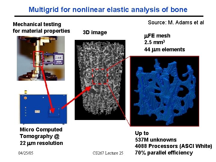
Methods: FE modeling Mechanical Testing E, yield, ult, etc. Source: Mark Adams, PPPL 3 D image FE mesh 2. 5 mm cube 44 m elements Micro-Computed Tomography CT @ 22 m resolution 04/25/05 CS 267 Lecture 25 Up to 537 M unknowns

Outline ° Recall Poisson Equation on regular mesh ° Recall solution by Multigrid ° Geometric Multigrid ° Algebraic Multigrid ° Software framework ° Numerical examples 04/25/05 CS 267 Lecture 25

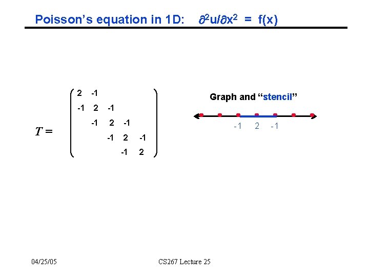
Poisson’s equation in 1 D: T= 04/25/05 2 -1 -1 2 2 u/ x 2 = f(x) Graph and “stencil” -1 CS 267 Lecture 25 2 -1

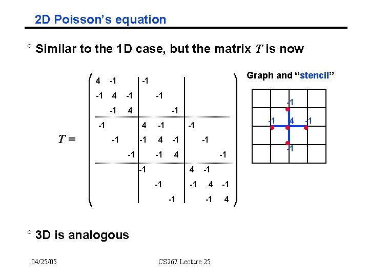
2 D Poisson’s equation ° Similar to the 1 D case, but the matrix T is now 4 -1 -1 4 -1 T= Graph and “stencil” -1 -1 -1 4 -1 -1 4 -1 -1 4 ° 3 D is analogous 04/25/05 CS 267 Lecture 25 4 -1 -1

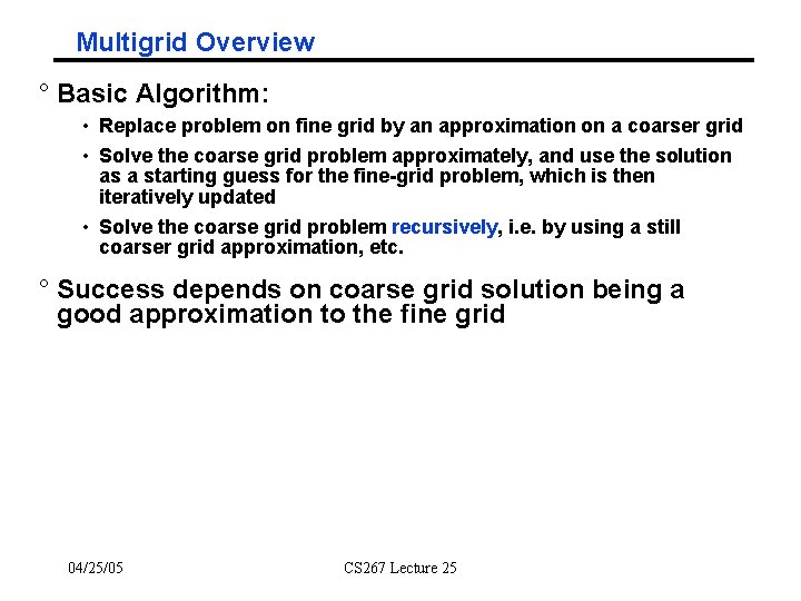
Multigrid Overview ° Basic Algorithm: • Replace problem on fine grid by an approximation on a coarser grid • Solve the coarse grid problem approximately, and use the solution as a starting guess for the fine-grid problem, which is then iteratively updated • Solve the coarse grid problem recursively, i. e. by using a still coarser grid approximation, etc. ° Success depends on coarse grid solution being a good approximation to the fine grid 04/25/05 CS 267 Lecture 25

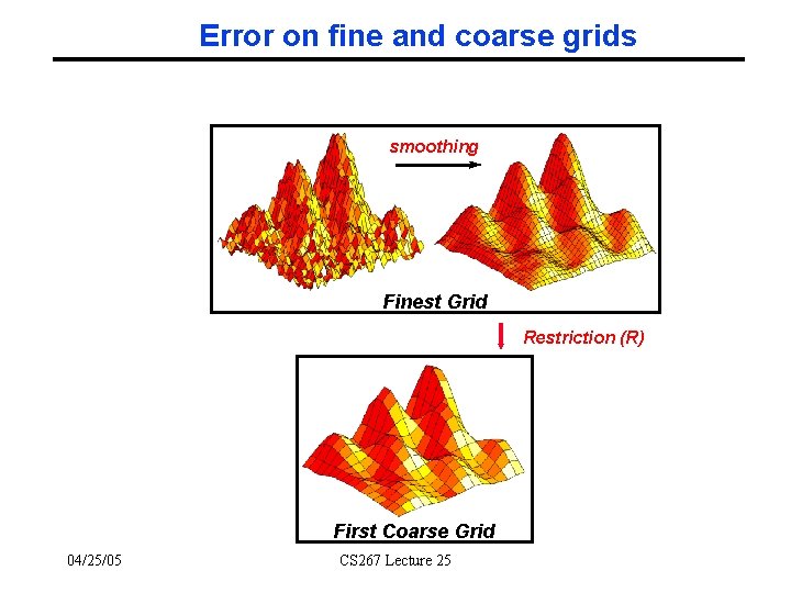
Error on fine and coarse grids smoothing Finest Grid Restriction (R) First Coarse Grid 04/25/05 CS 267 Lecture 25

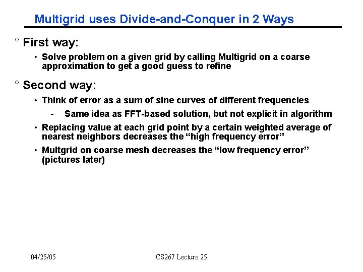
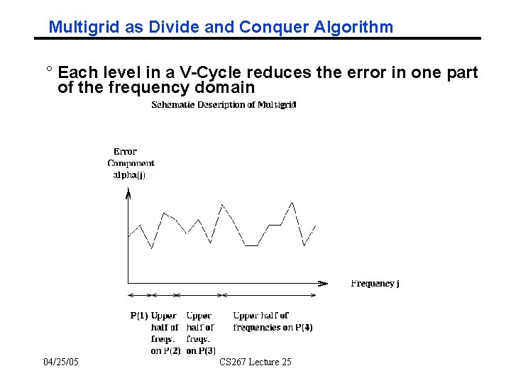
Multigrid uses Divide-and-Conquer in 2 Ways ° First way: • Solve problem on a given grid by calling Multigrid on a coarse approximation to get a good guess to refine ° Second way: • Think of error as a sum of sine curves of different frequencies - Same idea as FFT-based solution, but not explicit in algorithm • Replacing value at each grid point by a certain weighted average of nearest neighbors decreases the “high frequency error” • Multgrid on coarse mesh decreases the “low frequency error” (pictures later) 04/25/05 CS 267 Lecture 25

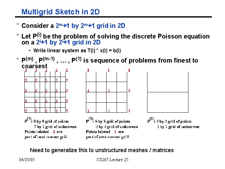
Multigrid Sketch in 2 D ° Consider a 2 m+1 by 2 m+1 grid in 2 D ° Let P(i) be the problem of solving the discrete Poisson equation on a 2 i+1 by 2 i+1 grid in 2 D • Write linear system as T(i) * x(i) = b(i) ° P(m) , P(m-1) , … , P(1) is sequence of problems from finest to coarsest Need to generalize this to unstructured meshes / matrices 04/25/05 CS 267 Lecture 25

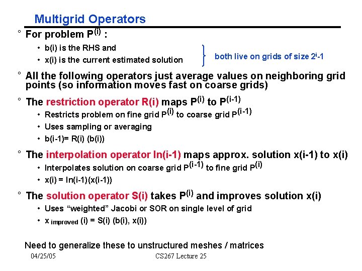
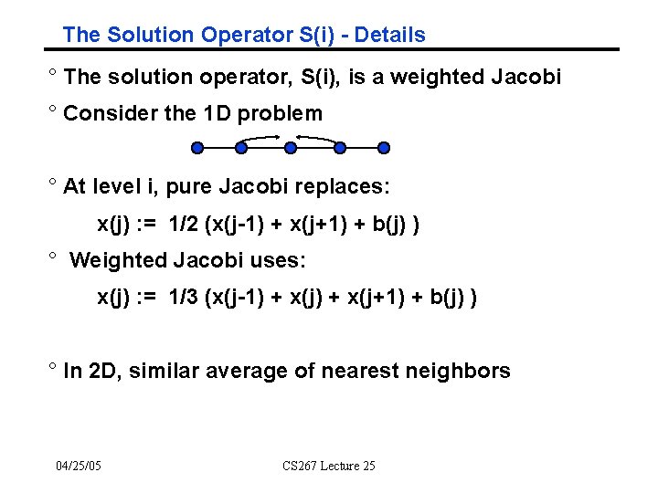
Multigrid Operators ° For problem P(i) : • b(i) is the RHS and • x(i) is the current estimated solution both live on grids of size 2 i-1 ° All the following operators just average values on neighboring grid points (so information moves fast on coarse grids) ° The restriction operator R(i) maps P(i) to P(i-1) • Restricts problem on fine grid P(i) to coarse grid P(i-1) • Uses sampling or averaging • b(i-1)= R(i) (b(i)) ° The interpolation operator In(i-1) maps approx. solution x(i-1) to x(i) • Interpolates solution on coarse grid P(i-1) to fine grid P(i) • x(i) = In(i-1)(x(i-1)) ° The solution operator S(i) takes P(i) and improves solution x(i) • Uses “weighted” Jacobi or SOR on single level of grid • x improved (i) = S(i) (b(i), x(i)) Need to generalize these to unstructured meshes / matrices 04/25/05 CS 267 Lecture 25

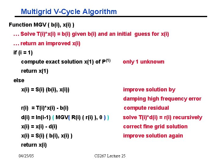
Multigrid V-Cycle Algorithm Function MGV ( b(i), x(i) ) … Solve T(i)*x(i) = b(i) given b(i) and an initial guess for x(i) … return an improved x(i) if (i = 1) compute exact solution x(1) of P(1) only 1 unknown return x(1) else x(i) = S(i) (b(i), x(i)) improve solution by damping high frequency error r(i) = T(i)*x(i) - b(i) compute residual d(i) = In(i-1) ( MGV( R(i) ( r(i) ), 0 ) ) solve T(i)*d(i) = r(i) recursively x(i) = x(i) - d(i) correct fine grid solution x(i) = S(i) ( b(i), x(i) ) improve solution again return x(i) 04/25/05 CS 267 Lecture 25

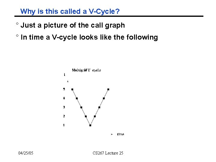
Why is this called a V-Cycle? ° Just a picture of the call graph ° In time a V-cycle looks like the following 04/25/05 CS 267 Lecture 25

The Solution Operator S(i) - Details ° The solution operator, S(i), is a weighted Jacobi ° Consider the 1 D problem ° At level i, pure Jacobi replaces: x(j) : = 1/2 (x(j-1) + x(j+1) + b(j) ) ° Weighted Jacobi uses: x(j) : = 1/3 (x(j-1) + x(j+1) + b(j) ) ° In 2 D, similar average of nearest neighbors 04/25/05 CS 267 Lecture 25

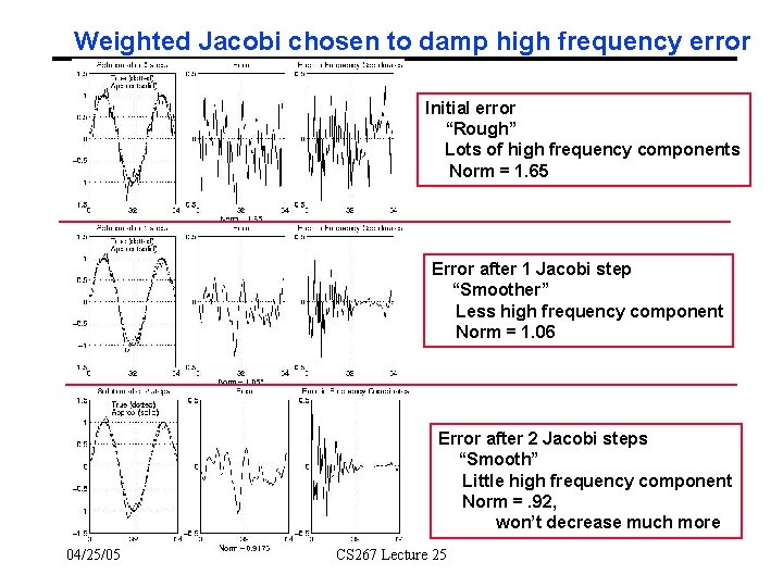
Weighted Jacobi chosen to damp high frequency error Initial error “Rough” Lots of high frequency components Norm = 1. 65 Error after 1 Jacobi step “Smoother” Less high frequency component Norm = 1. 06 Error after 2 Jacobi steps “Smooth” Little high frequency component Norm =. 92, won’t decrease much more 04/25/05 CS 267 Lecture 25

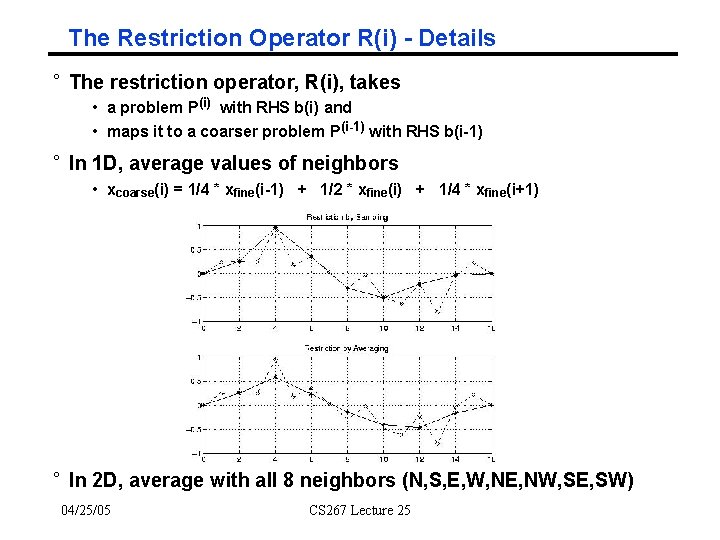
The Restriction Operator R(i) - Details ° The restriction operator, R(i), takes • a problem P(i) with RHS b(i) and • maps it to a coarser problem P(i-1) with RHS b(i-1) ° In 1 D, average values of neighbors • xcoarse(i) = 1/4 * xfine(i-1) + 1/2 * xfine(i) + 1/4 * xfine(i+1) ° In 2 D, average with all 8 neighbors (N, S, E, W, NE, NW, SE, SW) 04/25/05 CS 267 Lecture 25

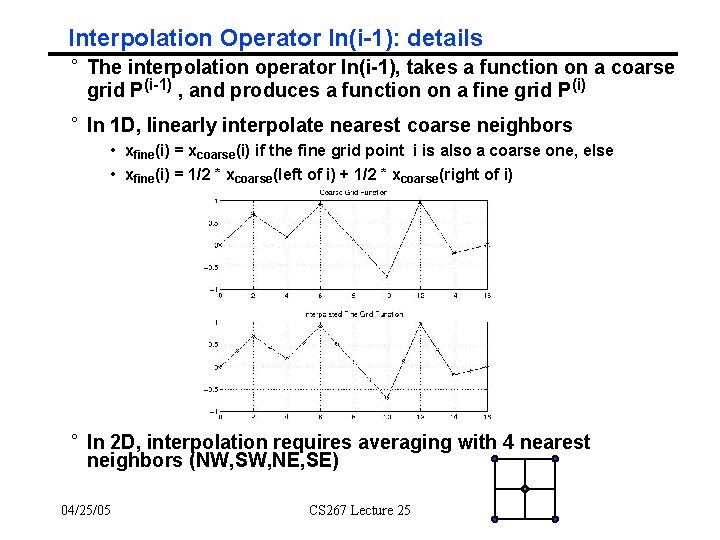
Interpolation Operator In(i-1): details ° The interpolation operator In(i-1), takes a function on a coarse grid P(i-1) , and produces a function on a fine grid P(i) ° In 1 D, linearly interpolate nearest coarse neighbors • xfine(i) = xcoarse(i) if the fine grid point i is also a coarse one, else • xfine(i) = 1/2 * xcoarse(left of i) + 1/2 * xcoarse(right of i) ° In 2 D, interpolation requires averaging with 4 nearest neighbors (NW, SW, NE, SE) 04/25/05 CS 267 Lecture 25

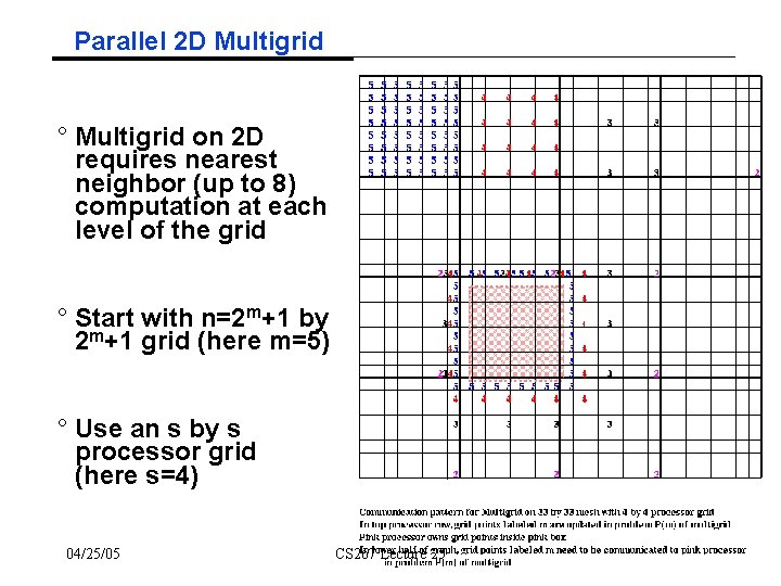
Parallel 2 D Multigrid ° Multigrid on 2 D requires nearest neighbor (up to 8) computation at each level of the grid ° Start with n=2 m+1 by 2 m+1 grid (here m=5) ° Use an s by s processor grid (here s=4) 04/25/05 CS 267 Lecture 25

Outline ° Recall Poisson Equation on regular mesh ° Recall solution by Multigrid ° Geometric Multigrid ° Algebraic Multigrid ° Software framework ° Numerical examples 04/25/05 CS 267 Lecture 25

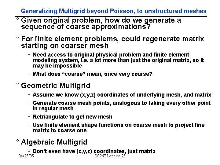
Generalizing Multigrid beyond Poisson, to unstructured meshes ° Given original problem, how do we generate a sequence of coarse approximations? ° For finite element problems, could regenerate matrix starting on coarser mesh • Need access to original physical problem and finite element modeling system, i. e. a lot more than just the original matrix, so it may be impossible • What does “coarse” mean, once very coarse? ° Geometric Multigrid • Assume we know (x, y, z) coordinates of underlying mesh, and matrix • Generate coarse mesh points, analogous to taking every other point in regular mesh • Retriangulate to get new mesh • Use finite element shape functions on coarse mesh to project fine matrix to coarse one ° Algebraic Multigrid • Don’t even have (x, y, z) coordinates, just matrix 04/25/05 CS 267 Lecture 25

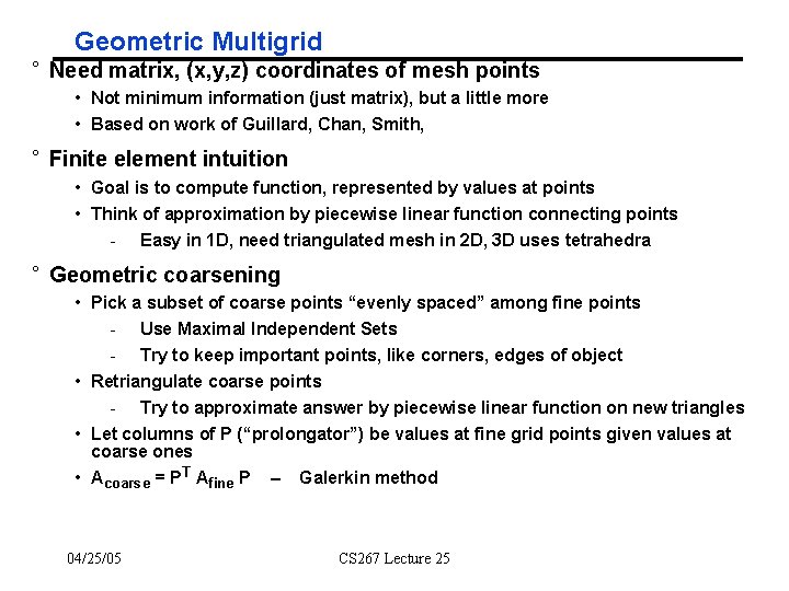
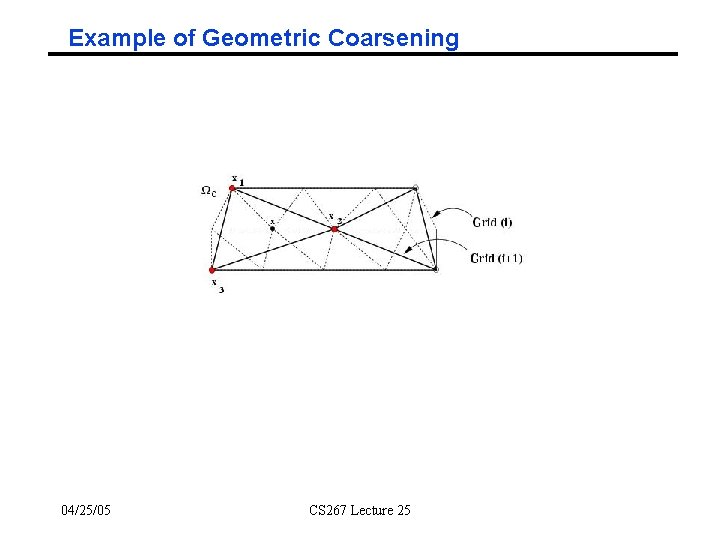
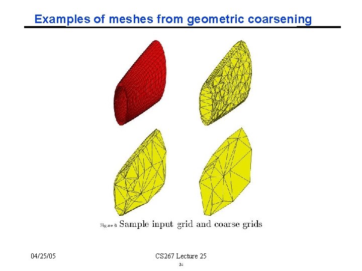
Geometric Multigrid ° Need matrix, (x, y, z) coordinates of mesh points • Not minimum information (just matrix), but a little more • Based on work of Guillard, Chan, Smith, ° Finite element intuition • Goal is to compute function, represented by values at points • Think of approximation by piecewise linear function connecting points - Easy in 1 D, need triangulated mesh in 2 D, 3 D uses tetrahedra ° Geometric coarsening • Pick a subset of coarse points “evenly spaced” among fine points - Use Maximal Independent Sets - Try to keep important points, like corners, edges of object • Retriangulate coarse points - Try to approximate answer by piecewise linear function on new triangles • Let columns of P (“prolongator”) be values at fine grid points given values at coarse ones • Acoarse = PT Afine P – Galerkin method 04/25/05 CS 267 Lecture 25

Example of Geometric Coarsening 04/25/05 CS 267 Lecture 25

Examples of meshes from geometric coarsening 04/25/05 CS 267 Lecture 25

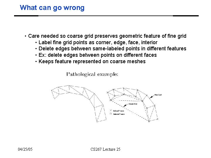
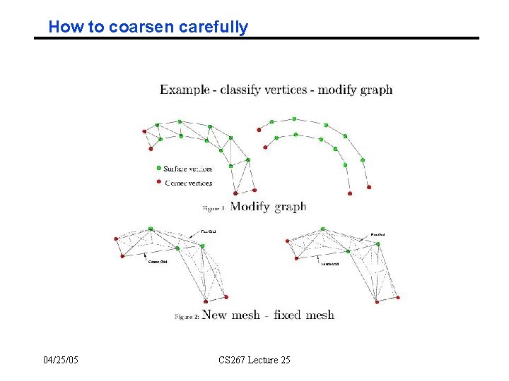
What can go wrong • Care needed so coarse grid preserves geometric feature of fine grid • Label fine grid points as corner, edge, face, interior • Delete edges between same-labeled points in different features • Ex: delete edges between points on different faces • Keeps feature represented on coarse meshes 04/25/05 CS 267 Lecture 25

How to coarsen carefully 04/25/05 CS 267 Lecture 25

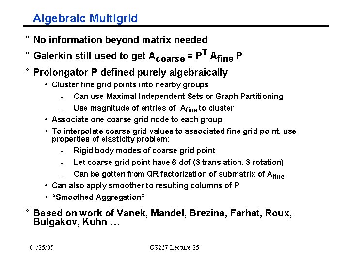
Algebraic Multigrid ° No information beyond matrix needed ° Galerkin still used to get Acoarse = PT Afine P ° Prolongator P defined purely algebraically • Cluster fine grid points into nearby groups - Can use Maximal Independent Sets or Graph Partitioning - Use magnitude of entries of Afine to cluster • Associate one coarse grid node to each group • To interpolate coarse grid values to associated fine grid point, use properties of elasticity problem: - Rigid body modes of coarse grid point - Let coarse grid point have 6 dof (3 translation, 3 rotation) - Can be gotten from QR factorization of submatrix of Afine • Can also apply smoother to resulting columns of P • “Smoothed Aggregation” ° Based on work of Vanek, Mandel, Brezina, Farhat, Roux, Bulgakov, Kuhn … 04/25/05 CS 267 Lecture 25

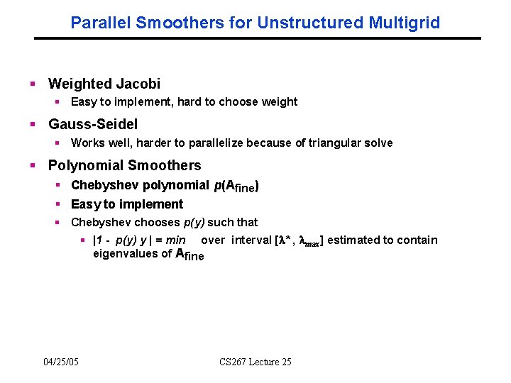
Parallel Smoothers for Unstructured Multigrid § Weighted Jacobi § Easy to implement, hard to choose weight § Gauss-Seidel § Works well, harder to parallelize because of triangular solve § Polynomial Smoothers § Chebyshev polynomial p(Afine) § Easy to implement § Chebyshev chooses p(y) such that § |1 - p(y) y | = min over interval [ * , max] estimated to contain eigenvalues of Afine 04/25/05 CS 267 Lecture 25

Outline ° Recall Poisson Equation on regular mesh ° Recall solution by Multigrid ° Geometric Multigrid ° Algebraic Multigrid ° Software framework ° Numerical examples 04/25/05 CS 267 Lecture 25

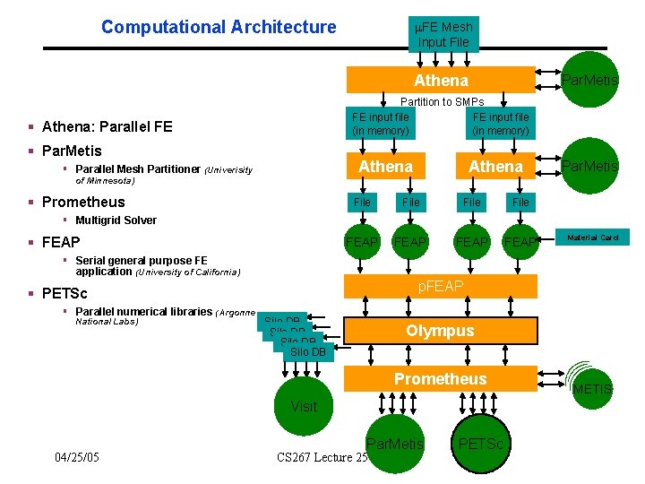
Computational Architecture FE Mesh Input File Athena Par. Metis Partition to SMPs FE input file (in memory) § Athena: Parallel FE § Par. Metis Athena § Parallel Mesh Partitioner (Univerisity of Minnesota) § Prometheus Athena File FEAP Par. Metis § Multigrid Solver § FEAP Material Card § Serial general purpose FE application (University of California) p. FEAP § PETSc § Parallel numerical libraries (Argonne National Labs) Silo DB Olympus Prometheus Visit 04/25/05 Par. Metis CS 267 Lecture 25 PETSc METIS

Outline ° Recall Poisson Equation on regular mesh ° Recall solution by Multigrid ° Geometric Multigrid ° Algebraic Multigrid ° Software framework ° Numerical examples • Work of Mark Adams • Scaled Speedup 04/25/05 CS 267 Lecture 25

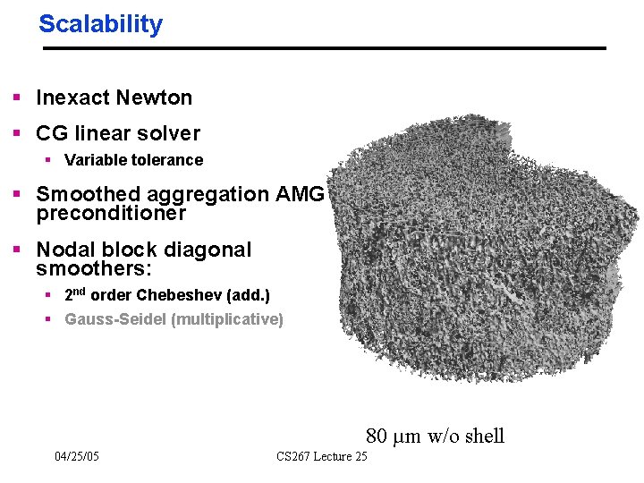
Scalability § Inexact Newton § CG linear solver § Variable tolerance § Smoothed aggregation AMG preconditioner § Nodal block diagonal smoothers: § 2 nd order Chebeshev (add. ) § Gauss-Seidel (multiplicative) 80 µm w/o shell 04/25/05 CS 267 Lecture 25

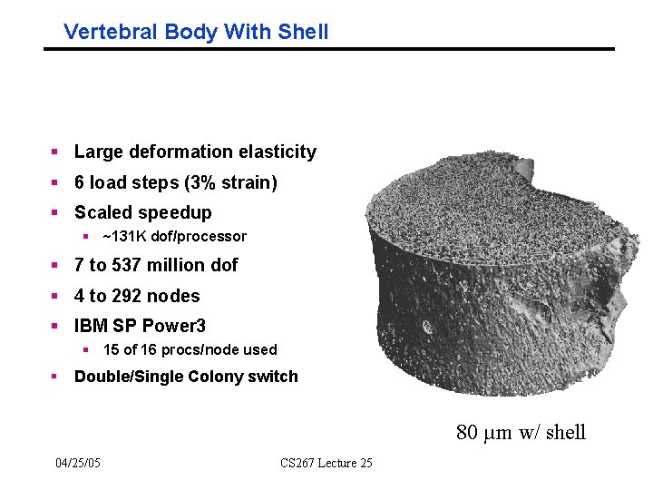
Vertebral Body With Shell § Large deformation elasticity § 6 load steps (3% strain) § Scaled speedup § ~131 K dof/processor § 7 to 537 million dof § 4 to 292 nodes § IBM SP Power 3 § 15 of 16 procs/node used § Double/Single Colony switch 80 µm w/ shell 04/25/05 CS 267 Lecture 25

Computational phases § Mesh setup (per mesh): § Coarse grid construction (aggregation) § Graph processing § Matrix setup (per matrix): § Coarse grid operator construction § Sparse matrix triple product PTAP § Subdomain factorizations § Solve (per RHS): § Matrix vector products (residuals, grid transfer) § Smoothers (Matrix vector products) 04/25/05 CS 267 Lecture 25

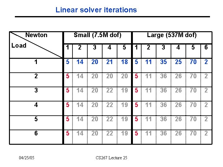
Linear solver iterations Newton Load 04/25/05 Small (7. 5 M dof) Large (537 M dof) 1 2 3 4 5 6 1 5 14 20 21 18 5 11 35 25 70 2 2 5 14 20 20 20 5 11 36 26 70 2 3 5 14 20 22 19 5 11 36 26 70 2 4 5 14 20 22 19 5 11 36 26 70 2 5 5 14 20 22 19 5 11 36 26 70 2 6 5 14 20 22 19 5 11 36 26 70 2 CS 267 Lecture 25

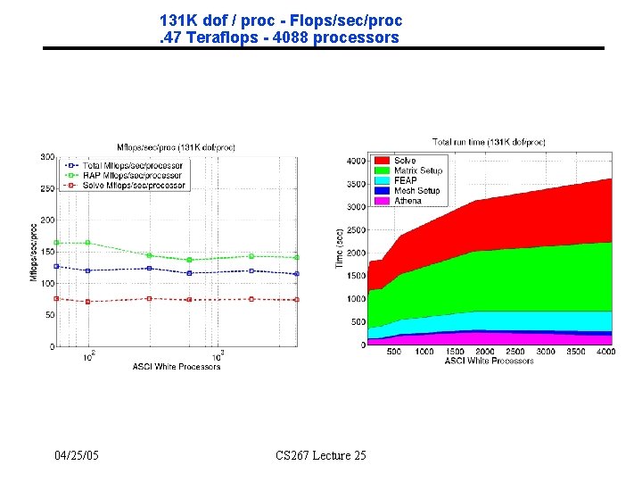
131 K dof / proc - Flops/sec/proc. 47 Teraflops - 4088 processors 04/25/05 CS 267 Lecture 25

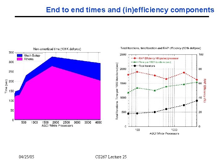
End to end times and (in)efficiency components 04/25/05 CS 267 Lecture 25

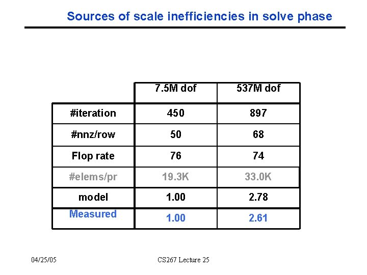
Sources of scale inefficiencies in solve phase 04/25/05 7. 5 M dof 537 M dof #iteration 450 897 #nnz/row 50 68 Flop rate 76 74 #elems/pr 19. 3 K 33. 0 K model 1. 00 2. 78 Measured 1. 00 2. 61 CS 267 Lecture 25

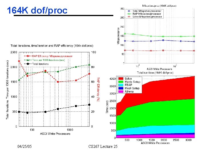
164 K dof/proc 04/25/05 CS 267 Lecture 25

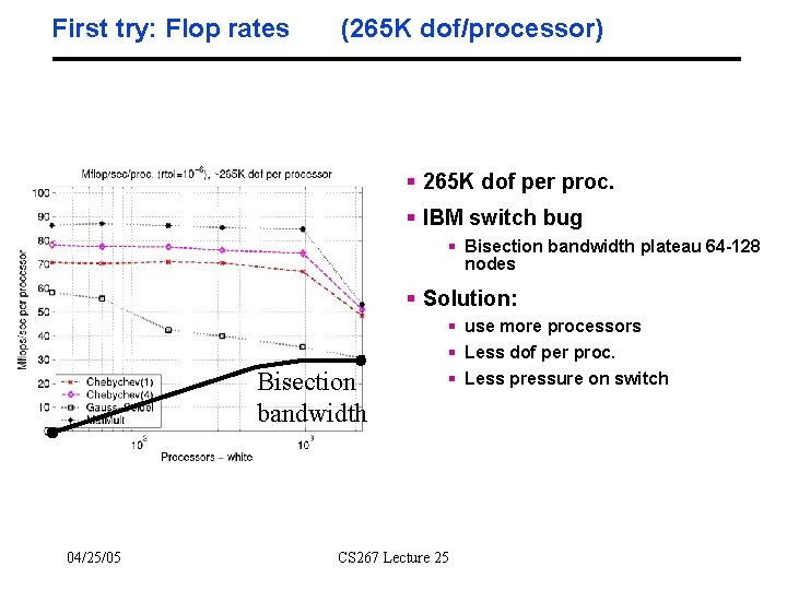
First try: Flop rates (265 K dof/processor) § 265 K dof per proc. § IBM switch bug § Bisection bandwidth plateau 64 -128 nodes § Solution: Bisection bandwidth 04/25/05 § use more processors § Less dof per proc. § Less pressure on switch CS 267 Lecture 25

Outline ° Recall Poisson Equation on regular mesh ° Recall solution by Multigrid ° Geometric Multigrid ° Algebraic Multigrid ° Software framework ° Numerical examples • Supplied by Mark Adams • Scaled Speedup • Plain Speedup 04/25/05 CS 267 Lecture 25

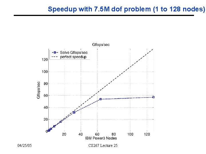
Speedup with 7. 5 M dof problem (1 to 128 nodes) 04/25/05 CS 267 Lecture 25

Outline ° Recall Poisson Equation on regular mesh ° Recall solution by Multigrid ° Geometric Multigrid ° Algebraic Multigrid ° Software framework ° Numerical examples • • Supplied by Mark Adams Scaled Speedup Plain Speedup Nodal Performance 04/25/05 CS 267 Lecture 25

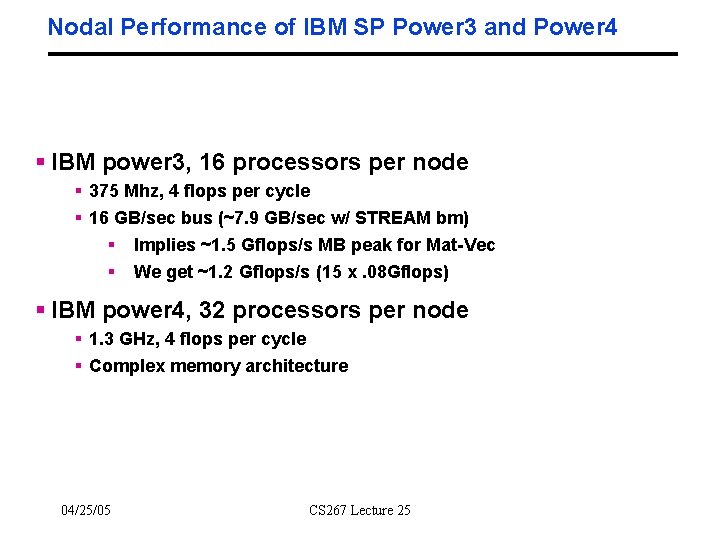
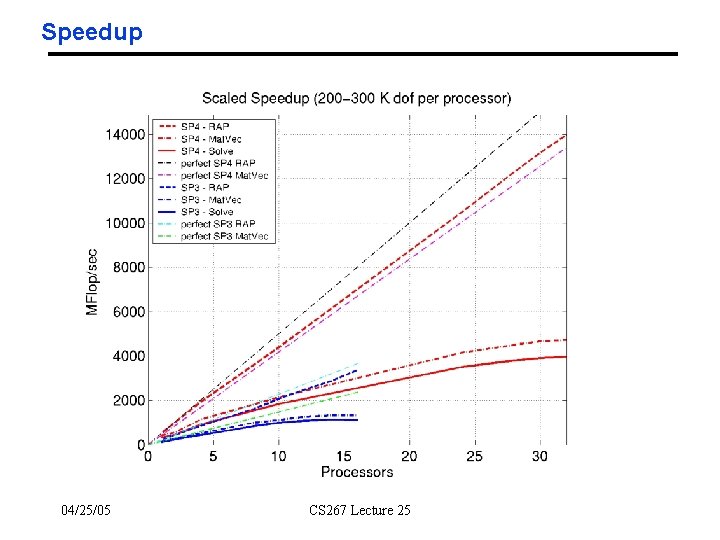
Nodal Performance of IBM SP Power 3 and Power 4 § IBM power 3, 16 processors per node § 375 Mhz, 4 flops per cycle § 16 GB/sec bus (~7. 9 GB/sec w/ STREAM bm) § Implies ~1. 5 Gflops/s MB peak for Mat-Vec § We get ~1. 2 Gflops/s (15 x. 08 Gflops) § IBM power 4, 32 processors per node § 1. 3 GHz, 4 flops per cycle § Complex memory architecture 04/25/05 CS 267 Lecture 25

Speedup 04/25/05 CS 267 Lecture 25

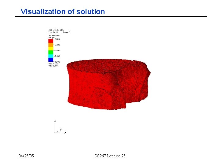
Visualization of solution 04/25/05 CS 267 Lecture 25

Conclusions ° Highly scalable solver for elasticity problems in complex geometries ° Built with mostly standard software tools • PETSc • Par. METIS • FEAP ° Winner of Gordon Bell Prize at Supercomputing 2004 ° See www. cs. berkeley. edu/~madams for more details 04/25/05 CS 267 Lecture 25

Extra Slides 04/25/05 CS 267 Lecture 25

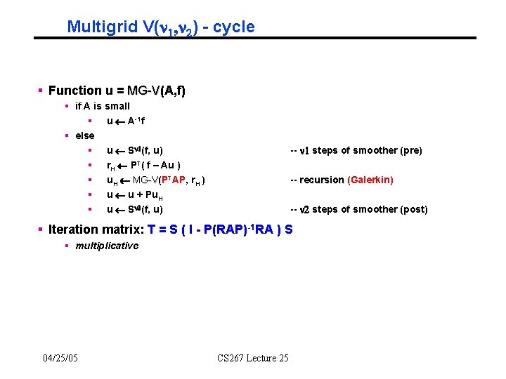
Multigrid V(n 1, n 2) - cycle § Function u = MG-V(A, f) MG-V § if A is small § u A-1 f § else § u Sn 1(f, u) § r. H PT( f – Au ) § u. H MG-V(P MG-V TAP, r. H ) § u u + Pu. H § u Sn 2(f, u) -- n 1 steps of smoother (pre) -- recursion (Galerkin) -- n 2 steps of smoother (post) § Iteration matrix: T = S ( I - P(RAP)-1 RA ) S § multiplicative 04/25/05 CS 267 Lecture 25

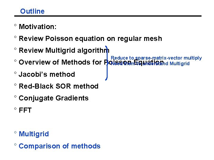
Outline ° Motivation: ° Review Poisson equation on regular mesh ° Review Multigrid algorithm ° Overview of Methods for ° Jacobi’s method ° Red-Black SOR method ° Conjugate Gradients ° FFT ° Multigrid ° Comparison of methods Reduce to sparse-matrix-vector multiply Poisson Need them. Equation to understand Multigrid

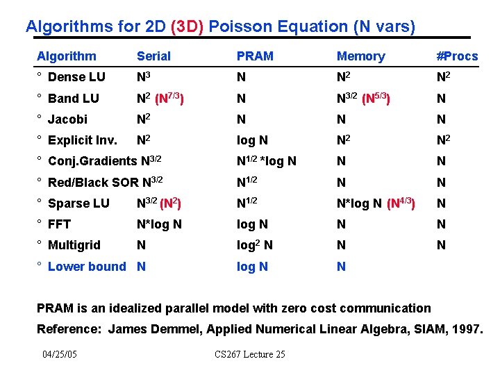
Algorithms for 2 D (3 D) Poisson Equation (N vars) Algorithm Serial PRAM Memory #Procs ° Dense LU N 3 N N 2 ° Band LU N 2 (N 7/3) N N 3/2 (N 5/3) N ° Jacobi N 2 N N N ° Explicit Inv. N 2 log N N 2 ° Conj. Gradients N 3/2 N 1/2 *log N N N ° Red/Black SOR N 3/2 N 1/2 N N ° Sparse LU N 3/2 (N 2) N 1/2 N*log N (N 4/3) N ° FFT N*log N N N ° Multigrid N log 2 N N N log N N ° Lower bound N PRAM is an idealized parallel model with zero cost communication Reference: James Demmel, Applied Numerical Linear Algebra, SIAM, 1997. 04/25/05 CS 267 Lecture 25

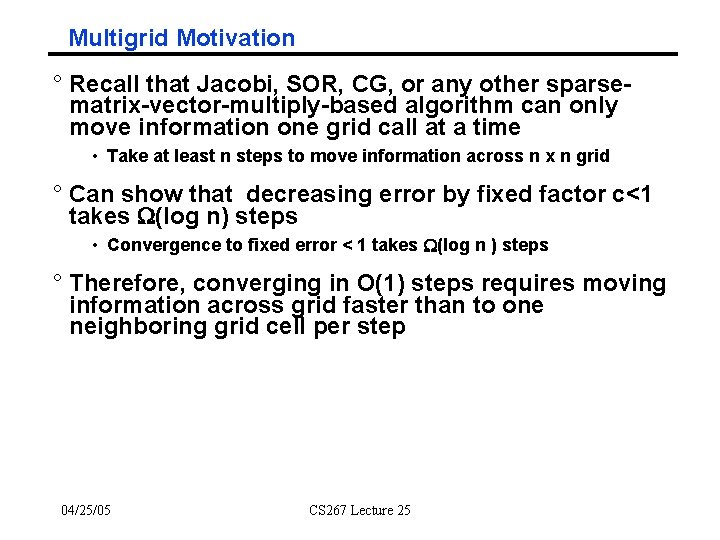
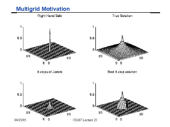
Multigrid Motivation ° Recall that Jacobi, SOR, CG, or any other sparsematrix-vector-multiply-based algorithm can only move information one grid call at a time • Take at least n steps to move information across n x n grid ° Can show that decreasing error by fixed factor c<1 takes W(log n) steps • Convergence to fixed error < 1 takes W(log n ) steps ° Therefore, converging in O(1) steps requires moving information across grid faster than to one neighboring grid cell per step 04/25/05 CS 267 Lecture 25

Multigrid Motivation 04/25/05 CS 267 Lecture 25

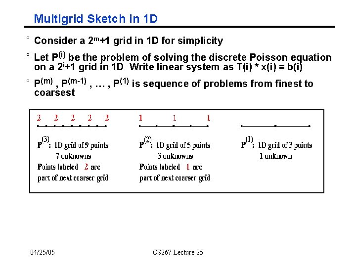
Multigrid Sketch in 1 D ° Consider a 2 m+1 grid in 1 D for simplicity ° Let P(i) be the problem of solving the discrete Poisson equation on a 2 i+1 grid in 1 D Write linear system as T(i) * x(i) = b(i) ° P(m) , P(m-1) , … , P(1) is sequence of problems from finest to coarsest 04/25/05 CS 267 Lecture 25

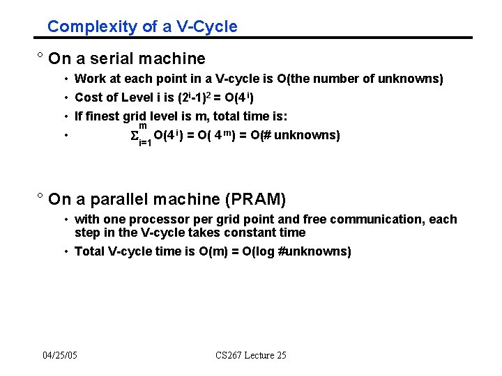
Complexity of a V-Cycle ° On a serial machine • Work at each point in a V-cycle is O(the number of unknowns) • Cost of Level i is (2 i-1)2 = O(4 i) • If finest grid level is m, total time is: m • S O(4 i) = O( 4 m) = O(# unknowns) i=1 ° On a parallel machine (PRAM) • with one processor per grid point and free communication, each step in the V-cycle takes constant time • Total V-cycle time is O(m) = O(log #unknowns) 04/25/05 CS 267 Lecture 25

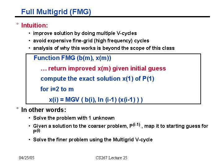
Full Multigrid (FMG) ° Intuition: • improve solution by doing multiple V-cycles • avoid expensive fine-grid (high frequency) cycles • analysis of why this works is beyond the scope of this class Function FMG (b(m), x(m)) … return improved x(m) given initial guess compute the exact solution x(1) of P(1) for i=2 to m x(i) = MGV ( b(i), In (i-1) (x(i-1) ) ) ° In other words: • Solve the problem with 1 unknown • Given a solution to the coarser problem, P(i-1) , map it to starting guess for P(i) • Solve the finer problem using the Multigrid V-cycle 04/25/05 CS 267 Lecture 25

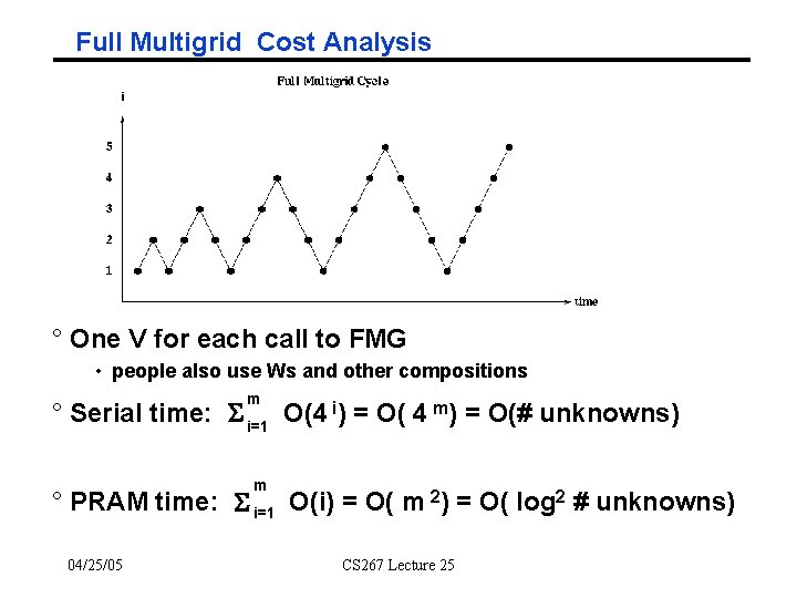
Full Multigrid Cost Analysis ° One V for each call to FMG • people also use Ws and other compositions m ° Serial time: S i=1 O(4 i) = O( 4 m) = O(# unknowns) m ° PRAM time: S i=1 O(i) = O( m 2) = O( log 2 # unknowns) 04/25/05 CS 267 Lecture 25

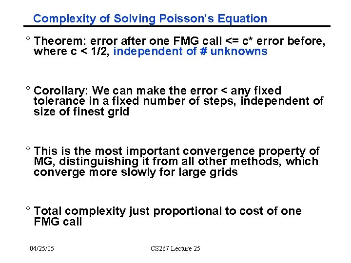
Complexity of Solving Poisson’s Equation ° Theorem: error after one FMG call <= c* error before, where c < 1/2, independent of # unknowns ° Corollary: We can make the error < any fixed tolerance in a fixed number of steps, independent of size of finest grid ° This is the most important convergence property of MG, distinguishing it from all other methods, which converge more slowly for large grids ° Total complexity just proportional to cost of one FMG call 04/25/05 CS 267 Lecture 25

Multigrid as Divide and Conquer Algorithm ° Each level in a V-Cycle reduces the error in one part of the frequency domain 04/25/05 CS 267 Lecture 25

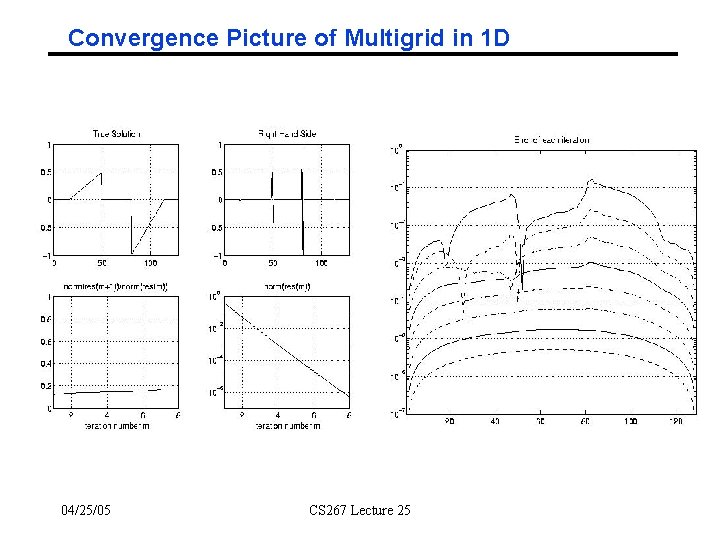
Convergence Picture of Multigrid in 1 D 04/25/05 CS 267 Lecture 25

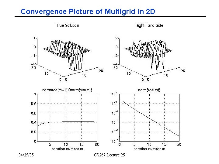
Convergence Picture of Multigrid in 2 D 04/25/05 CS 267 Lecture 25

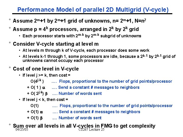
Performance Model of parallel 2 D Multigrid (V-cycle) ° Assume 2 m+1 by 2 m+1 grid of unknowns, n= 2 m+1, N=n 2 ° Assume p = 4 k processors, arranged in 2 k by 2 k grid • Each processor starts with 2 m-k by 2 m-k subgrid of unknowns ° Consider V-cycle starting at level m • At levels m through k of V-cycle, each processor does some work • At levels k-1 through 1, some processors are idle, because a 2 k-1 by 2 k-1 grid of unknowns cannot occupy each processor ° Cost of one level in V-cycle • If level j >= k, then cost = O(4 j-k ) …. Flops, proportional to the number of grid points/processor + O( 1 ) a …. Send a constant # messages to neighbors + O( 2 j-k) b …. Number of words sent • If level j < k, then cost = O(1) …. Flops, proportional to the number of grid points/processor + O(1) a …. Send a constant # messages to neighbors + O(1) b. … Number of words sent ° Sum over all levels in all V-cycles in FMG to get complexity 04/25/05 CS 267 Lecture 25

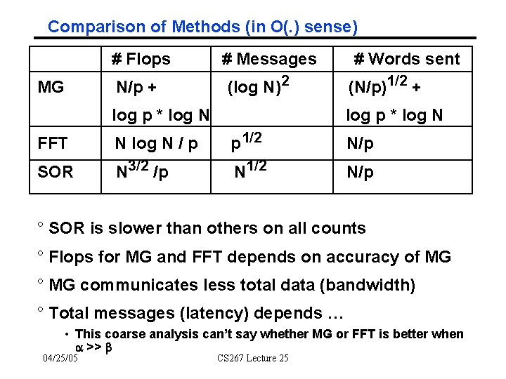
Comparison of Methods (in O(. ) sense) # Flops MG N/p + # Messages (log N)2 log p * log N # Words sent (N/p)1/2 + log p * log N FFT N log N / p p 1/2 N/p SOR N 3/2 /p N 1/2 N/p ° SOR is slower than others on all counts ° Flops for MG and FFT depends on accuracy of MG ° MG communicates less total data (bandwidth) ° Total messages (latency) depends … • This coarse analysis can’t say whether MG or FFT is better when a >> b 04/25/05 CS 267 Lecture 25

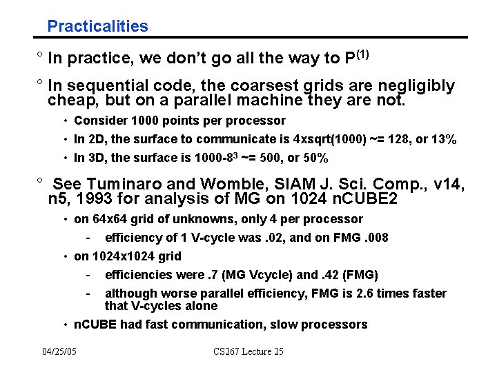
Practicalities ° In practice, we don’t go all the way to P(1) ° In sequential code, the coarsest grids are negligibly cheap, but on a parallel machine they are not. • Consider 1000 points per processor • In 2 D, the surface to communicate is 4 xsqrt(1000) ~= 128, or 13% • In 3 D, the surface is 1000 -83 ~= 500, or 50% ° See Tuminaro and Womble, SIAM J. Sci. Comp. , v 14, n 5, 1993 for analysis of MG on 1024 n. CUBE 2 • on 64 x 64 grid of unknowns, only 4 per processor - efficiency of 1 V-cycle was. 02, and on FMG. 008 • on 1024 x 1024 grid - efficiencies were. 7 (MG Vcycle) and. 42 (FMG) - although worse parallel efficiency, FMG is 2. 6 times faster that V-cycles alone • n. CUBE had fast communication, slow processors 04/25/05 CS 267 Lecture 25

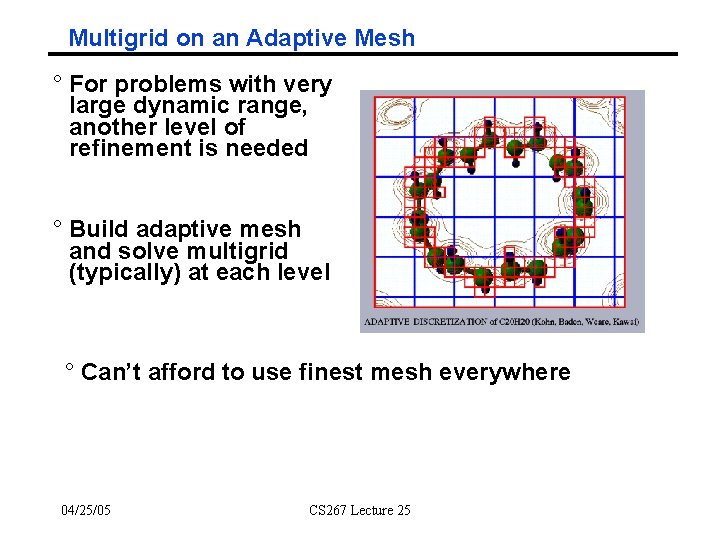
Multigrid on an Adaptive Mesh ° For problems with very large dynamic range, another level of refinement is needed ° Build adaptive mesh and solve multigrid (typically) at each level ° Can’t afford to use finest mesh everywhere 04/25/05 CS 267 Lecture 25

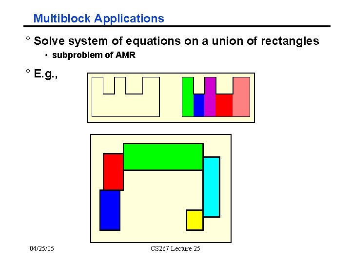
Multiblock Applications ° Solve system of equations on a union of rectangles • subproblem of AMR ° E. g. , 04/25/05 CS 267 Lecture 25

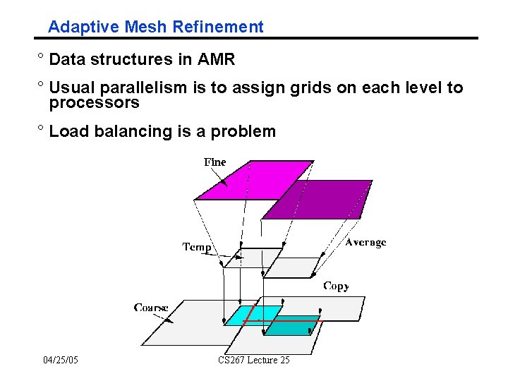
Adaptive Mesh Refinement ° Data structures in AMR ° Usual parallelism is to assign grids on each level to processors ° Load balancing is a problem 04/25/05 CS 267 Lecture 25

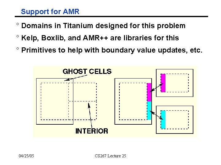
Support for AMR ° Domains in Titanium designed for this problem ° Kelp, Boxlib, and AMR++ are libraries for this ° Primitives to help with boundary value updates, etc. 04/25/05 CS 267 Lecture 25

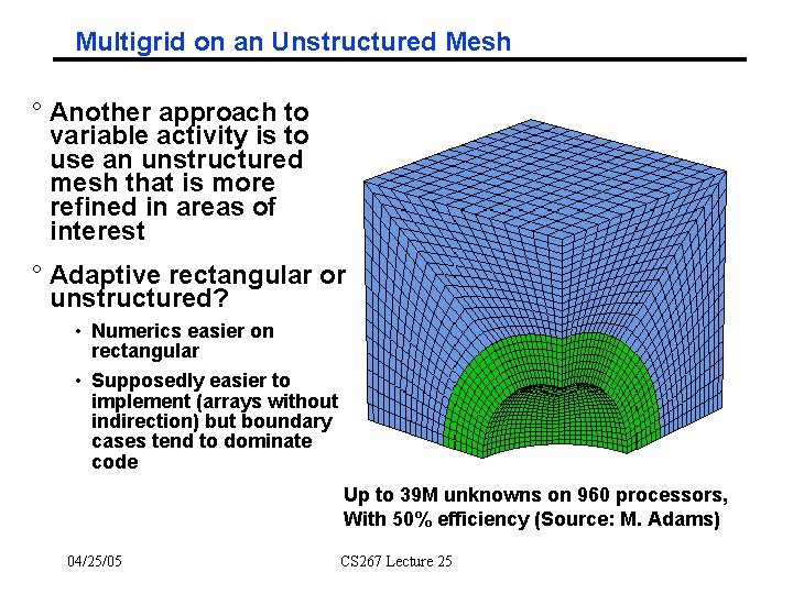
Multigrid on an Unstructured Mesh ° Another approach to variable activity is to use an unstructured mesh that is more refined in areas of interest ° Adaptive rectangular or unstructured? • Numerics easier on rectangular • Supposedly easier to implement (arrays without indirection) but boundary cases tend to dominate code Up to 39 M unknowns on 960 processors, With 50% efficiency (Source: M. Adams) 04/25/05 CS 267 Lecture 25

Multigrid on an Unstructured Mesh ° Need to partition graph for parallelism ° What does it mean to do Multigrid anyway? ° Need to be able to coarsen grid (hard problem) • Can’t just pick “every other grid point” anymore • Use “maximal independent sets” again • How to make coarse graph approximate fine one ° Need to define R() and In() • How do we convert from coarse to fine mesh and back? ° Need to define S() • How do we define coarse matrix (no longer formula, like Poisson) ° Dealing with coarse meshes efficiently • Should we switch to using fewer processors on coarse meshes? • Should we switch to another solver on coarse meshes? 04/25/05 CS 267 Lecture 25

Trabecular Bone: Failure modes under stress Cortical bone Trabecular bone 04/25/05 CS 267 Lecture 25 5 -mm Cube Source: Mark Adams, PPPL

Multigrid for nonlinear elastic analysis of bone Mechanical testing for material properties Source: M. Adams et al 3 D image FE mesh 2. 5 mm 3 44 m elements Micro Computed Tomography @ 22 m resolution 04/25/05 CS 267 Lecture 25 Up to 537 M unknowns 4088 Processors (ASCI White) 70% parallel efficiency