CS 244 Introduction to Embedded Systems and Ubiquitous

CS 244 -Introduction to Embedded Systems and Ubiquitous Computing Instructor: Eli Bozorgzadeh Computer Science Department UC Irvine Winter 2010

CS 244 – Lecture 6 Model of Computation Winter 2010 - CS 244 2

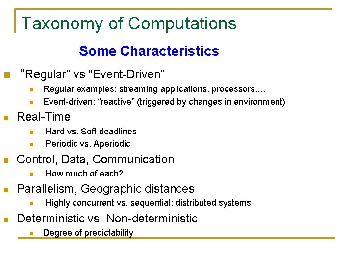
Taxonomy of Computations Some Characteristics n “Regular” vs “Event-Driven” n n n Real-Time n n n How much of each? Parallelism, Geographic distances n n Hard vs. Soft deadlines Periodic vs. Aperiodic Control, Data, Communication n n Regular examples: streaming applications, processors, … Event-driven: “reactive” (triggered by changes in environment) Highly concurrent vs. sequential; distributed systems Deterministic vs. Non-deterministic n Degree of predictability

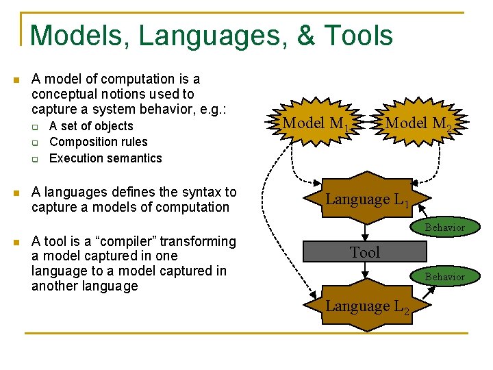
Models, Languages, & Tools n A model of computation is a conceptual notions used to capture a system behavior, e. g. : q q q n A set of objects Composition rules Execution semantics A languages defines the syntax to capture a models of computation Model M 1 Model M 2 Language L 1 Behavior n A tool is a “compiler” transforming a model captured in one language to a model captured in another language Tool Behavior Language L 2

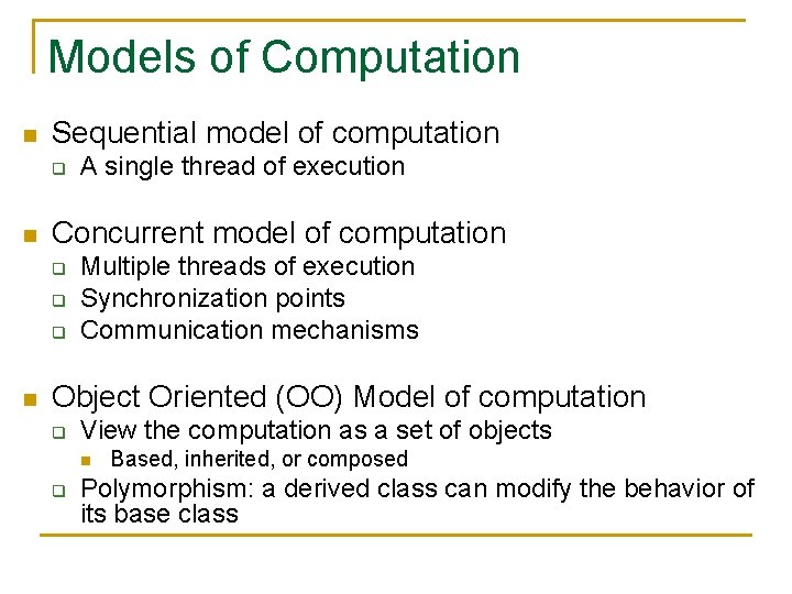
Models of Computation n Sequential model of computation q n Concurrent model of computation q q q n A single thread of execution Multiple threads of execution Synchronization points Communication mechanisms Object Oriented (OO) Model of computation q View the computation as a set of objects n q Based, inherited, or composed Polymorphism: a derived class can modify the behavior of its base class

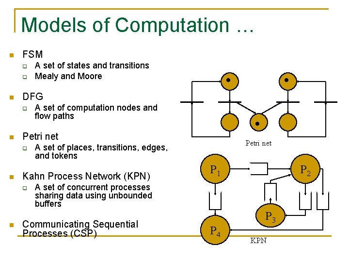
Models of Computation … n FSM q q n DFG q n Petri net A set of places, transitions, edges, and tokens Kahn Process Network (KPN) q n A set of computation nodes and flow paths Petri net q n A set of states and transitions Mealy and Moore P 1 P 2 A set of concurrent processes sharing data using unbounded buffers Communicating Sequential Processes (CSP) P 4 P 3 KPN

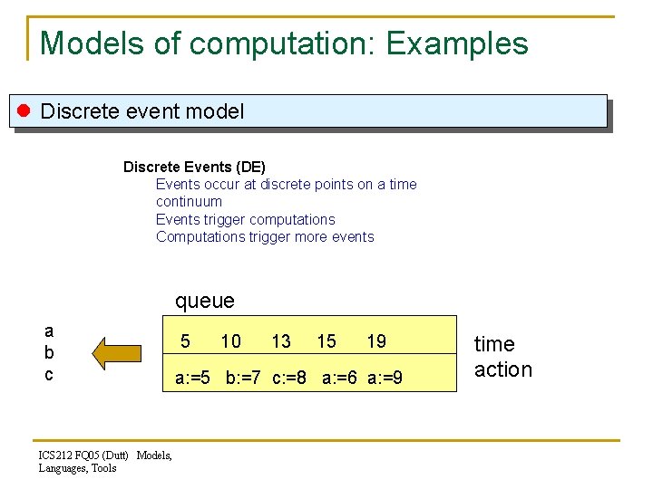
Models of computation: Examples l Discrete event model Discrete Events (DE) Events occur at discrete points on a time continuum Events trigger computations Computations trigger more events queue a b c ICS 212 FQ 05 (Dutt) Models, Languages, Tools 5 10 13 15 19 a: =5 b: =7 c: =8 a: =6 a: =9 time action

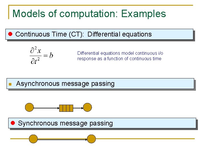
Models of computation: Examples l Continuous Time (CT): Differential equations model continuous i/o response as a function of continuous time n Asynchronous message passing l Synchronous message passing

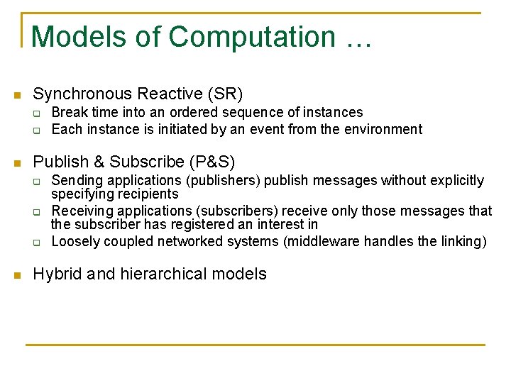
Models of Computation … n Synchronous Reactive (SR) q q n Publish & Subscribe (P&S) q q q n Break time into an ordered sequence of instances Each instance is initiated by an event from the environment Sending applications (publishers) publish messages without explicitly specifying recipients Receiving applications (subscribers) receive only those messages that the subscriber has registered an interest in Loosely coupled networked systems (middleware handles the linking) Hybrid and hierarchical models

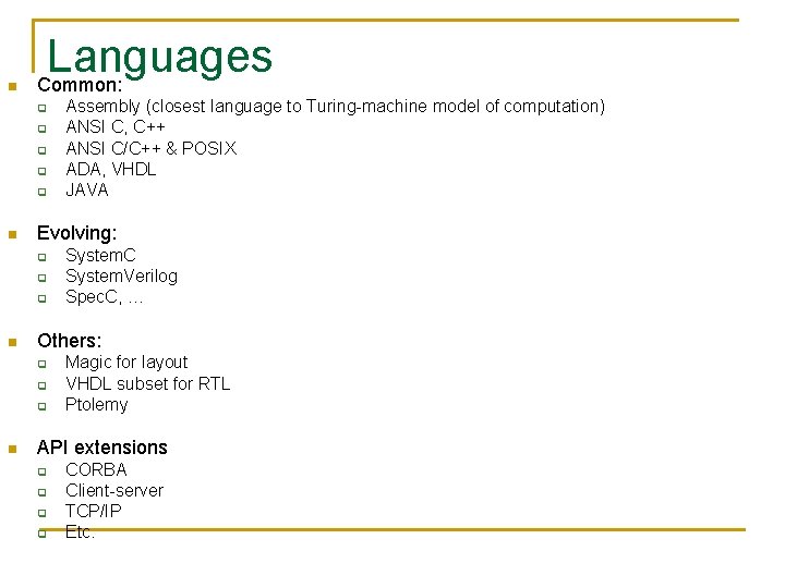
n Languages Common: q q q n Evolving: q q q n System. C System. Verilog Spec. C, … Others: q q q n Assembly (closest language to Turing-machine model of computation) ANSI C, C++ ANSI C/C++ & POSIX ADA, VHDL JAVA Magic for layout VHDL subset for RTL Ptolemy API extensions q q CORBA Client-server TCP/IP Etc.

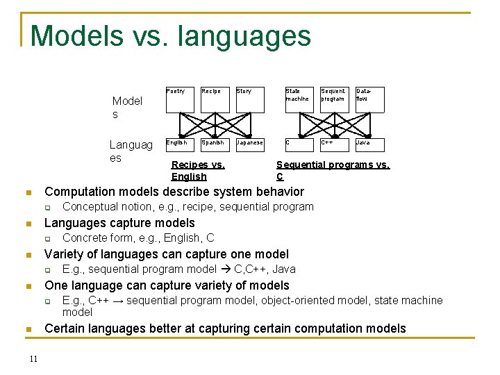
Models vs. languages Poetry Recipe Story State machine Sequent. program Dataflow English Spanish Japanese C C++ Java Model s Languag es n 11 E. g. , sequential program model C, C++, Java One language can capture variety of models q n Concrete form, e. g. , English, C Variety of languages can capture one model q n Conceptual notion, e. g. , recipe, sequential program Languages capture models q n Sequential programs vs. C Computation models describe system behavior q n Recipes vs. English E. g. , C++ → sequential program model, object-oriented model, state machine model Certain languages better at capturing certain computation models

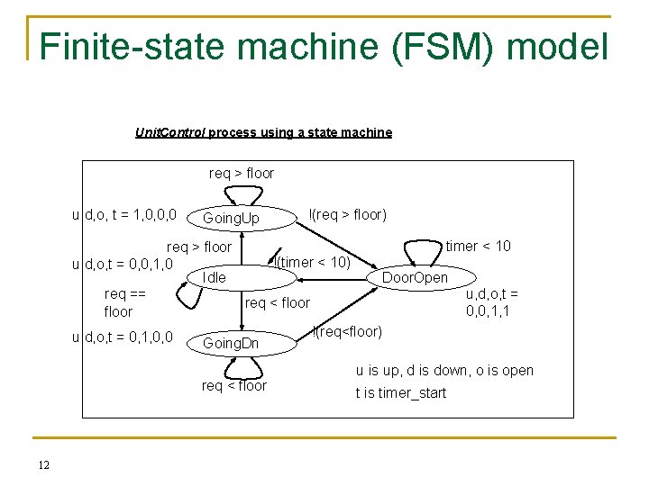
Finite-state machine (FSM) model Unit. Control process using a state machine req > floor u, d, o, t = 1, 0, 0, 0 Going. Up !(req > floor) timer < 10 req > floor !(timer < 10) u, d, o, t = 0, 0, 1, 0 Idle Door. Open u, d, o, t = req == req < floor 0, 0, 1, 1 floor !(req<floor) u, d, o, t = 0, 1, 0, 0 Going. Dn req < floor 12 u is up, d is down, o is open t is timer_start

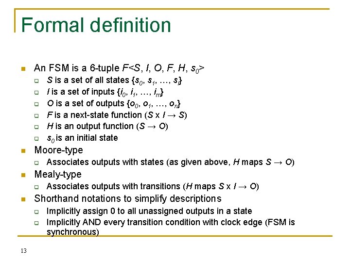
Formal definition n An FSM is a 6 -tuple F<S, I, O, F, H, s 0> q q q n Moore-type q n Associates outputs with transitions (H maps S x I → O) Shorthand notations to simplify descriptions q q 13 Associates outputs with states (as given above, H maps S → O) Mealy-type q n S is a set of all states {s 0, s 1, …, sl} I is a set of inputs {i 0, i 1, …, im} O is a set of outputs {o 0, o 1, …, on} F is a next-state function (S x I → S) H is an output function (S → O) s 0 is an initial state Implicitly assign 0 to all unassigned outputs in a state Implicitly AND every transition condition with clock edge (FSM is synchronous)

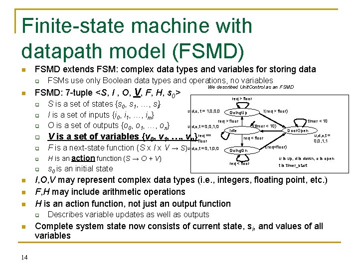
Finite-state machine with datapath model (FSMD) n FSMD extends FSM: complex data types and variables for storing data q n q q V is a set of variables {v 0, v 1, …, v } q q q n 14 u, d, o, t = 1, 0, 0, 0 Going. Up req > floor u, d, o, t = 0, 0, 1, 0 Idle req == n floor F is a next-state function (S x I x V → S)u, d, o, t = 0, 1, 0, 0 H is an action function (S → O + V) s 0 is an initial state !(req > floor) timer < 10 !(timer < 10) Door. Open req < floor Going. Dn req < floor u, d, o, t = 0, 0, 1, 1 !(req<floor) u is up, d is down, o is open t is timer_start I, O, V may represent complex data types (i. e. , integers, floating point, etc. ) F, H may include arithmetic operations H is an action function, not just an output function q n req > floor S is a set of states {s 0, s 1, …, sl} I is a set of inputs {i 0, i 1, …, im} O is a set of outputs {o 0, o 1, …, on} q n We described Unit. Control as an FSMD: 7 -tuple <S, I , O, V, F, H, s 0> q n FSMs use only Boolean data types and operations, no variables Describes variable updates as well as outputs Complete system state now consists of current state, si, and values of all variables

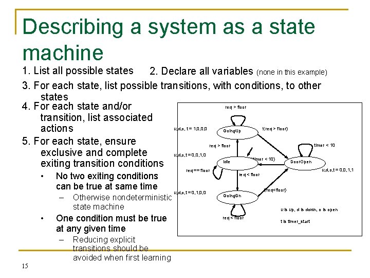
Describing a system as a state machine 1. List all possible states 2. Declare all variables (none in this example) 3. For each state, list possible transitions, with conditions, to other states req > floor 4. For each state and/or transition, list associated u, d, o, t = 1, 0, 0, 0 !(req > floor) actions Going. Up 5. For each state, ensure timer < 10 req > floor exclusive and complete u, d, o, t = 0, 0, 1, 0 !(timer < 10) Idle Door. Open exiting transition conditions u, d, o, t = 0, 0, 1, 1 req == floor • No two exiting conditions can be true at same time – • One condition must be true at any given time – 15 Otherwise nondeterministic state machine Reducing explicit transitions should be avoided when first learning req < floor u, d, o, t = 0, 1, 0, 0 !(req<floor) Going. Dn u is up, d is down, o is open req < floor t is timer_start

State machine vs. sequential program model n n Different thought process used with each model State machine: q n Sequential program model: q n Encourages designer to think of all possible states and transitions among states based on all possible input conditions Designed to transform data through series of instructions that may be iterated and conditionally executed State machine description excels in many cases q q More natural means of computing in those cases Not due to graphical representation (state diagram) n n 16 Would still have same benefits if textual language used (i. e. , state table) Besides, sequential program model could use graphical representation (i. e. , flowchart)

Try Capturing Other Behaviors with an FSM n n 17 E. g. , Answering machine blinking light when there are messages E. g. , A simple telephone answering machine that answers after 4 rings when activated E. g. , A simple crosswalk traffic control light Others

Capturing state machines in sequential programming language n Despite benefits of state machine model, most popular development tools use sequential programming language q q C, C++, Java, Ada, VHDL, Verilog, etc. Development tools are complex and expensive, therefore not easy to adapt or replace n n Must protect investment Two approaches to capturing state machine model with sequential programming language q Front-end tool approach n Additional tool installed to support state machine language q q q n q Drawback: must support additional tool (licensing costs, upgrades, training, etc. ) Language subset approach n 18 Graphical and/or textual state machine languages May support graphical simulation Automatically generate code in sequential programming language that is input to main development tool Most common approach. . .

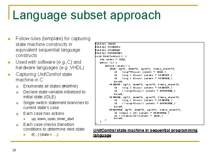
Language subset approach n n n Follow rules (template) for capturing state machine constructs in equivalent sequential language constructs Used with software (e. g. , C) and hardware languages (e. g. , VHDL) Capturing Unit. Control state machine in C q q Enumerate all states (#define) Declare state variable initialized to initial state (IDLE) Single switch statement branches to current state’s case Each case has actions n q Each case checks transition conditions to determine next state n 19 up, down, open, timer_start if(…) {state = …; } #define IDLE 0 #define GOINGUP 1 #define GOINGDN 2 #define DOOROPEN 3 void Unit. Control() { int state = IDLE; while (1) { switch (state) { IDLE: up=0; down=0; open=1; timer_start=0; if (req==floor) {state = IDLE; } if (req > floor) {state = GOINGUP; } if (req < floor) {state = GOINGDN; } break; GOINGUP: up=1; down=0; open=0; timer_start=0; if (req > floor) {state = GOINGUP; } if (!(req>floor)) {state = DOOROPEN; } break; GOINGDN: up=1; down=0; open=0; timer_start=0; if (req < floor) {state = GOINGDN; } if (!(req<floor)) {state = DOOROPEN; } break; DOOROPEN: up=0; down=0; open=1; timer_start=1; if (timer < 10) {state = DOOROPEN; } if (!(timer<10)){state = IDLE; } break; } } } Unit. Control state machine in sequential programming language

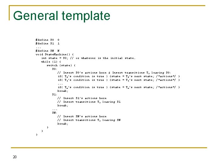
General template #define S 0 0 #define S 1 1. . . #define SN N void State. Machine() { int state = S 0; // or whatever is the initial state. while (1) { switch (state) { S 0: // Insert S 0’s actions here & Insert transitions Ti leaving S 0: if( T 0’s condition is true ) {state = T 0’s next state; /*actions*/ } if( T 1’s condition is true ) {state = T 1’s next state; /*actions*/ }. . . if( Tm’s condition is true ) {state = Tm’s next state; /*actions*/ } break; S 1: // Insert S 1’s actions here // Insert transitions Ti leaving S 1 break; . . . SN: // Insert SN’s actions here // Insert transitions Ti leaving SN break; } } } 20

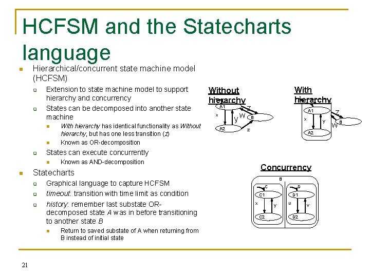
HCFSM and the Statecharts language n Hierarchical/concurrent state machine model (HCFSM) q q Extension to state machine model to support hierarchy and concurrency States can be decomposed into another state machine n n q yw x A 2 z B x z q q y A 2 Known as AND-decomposition Graphical language to capture HCFSM timeout: transition with time limit as condition history: remember last substate ORdecomposed state A was in before transitioning to another state B n Return to saved substate of A when returning from B instead of initial state z A 1 Concurrency Statecharts q 21 A 1 With hierarchy A States can execute concurrently n n With hierarchy has identical functionality as Without hierarchy, but has one less transition (z) Known as OR-decomposition Without hierarchy B C D C 1 x D 1 y C 2 u v D 2 w B

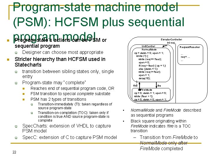
n Program-state machine model (PSM): HCFSM plus sequential program model Program-state’s actions can be FSM or Elevator. Controller int req; sequential program q n Unit. Control Normal. Mode up = down = 0; open = 1; while (1) { while (req == floor); open = 0; if (req > floor) { up = 1; } else {down = 1; } while (req != floor); open = 1; delay(10); } !fire} fire Designer can choose most appropriate Stricter hierarchy than HCFSM used in Statecharts q q transition between sibling states only, single entry Program-state may “complete” n n n Reaches end of sequential program code, OR FSM transition to special complete substate PSM has 2 types of transitions q q 22 Transition-immediately (TI): taken regardless of source program-state Transition-on-completion (TOC): taken only if condition is true AND source program-state is complete Spec. Charts: extension of VHDL to capture PSM model Spec. C: extension of C to capture PSM model Request. Resolver. . . req =. . . Fire. Mode up = 0; down = 1; open = 0; while (floor > 1); up = 0; down = 0; open = 1; • • Normal. Mode and Fire. Mode described as sequential programs Black square originating within Fire. Mode indicates !fire is a TOC transition – Transition from Fire. Mode to Normal. Mode only after Fire. Mode completed

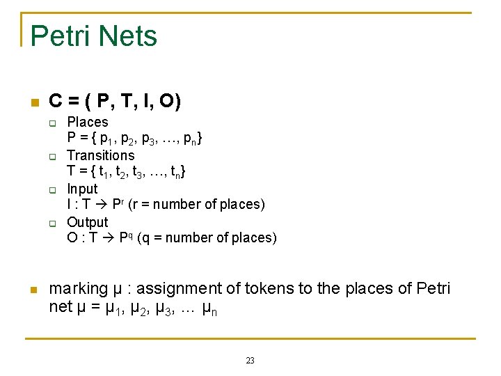
Petri Nets n C = ( P, T, I, O) q q n Places P = { p 1, p 2, p 3, …, pn} Transitions T = { t 1, t 2, t 3, …, tn} Input I : T Pr (r = number of places) Output O : T Pq (q = number of places) marking µ : assignment of tokens to the places of Petri net µ = µ 1, µ 2, µ 3, … µn 23

Applications of Petri Net n Petri net is primarily used for studying the dynamic concurrent behavior of network-based systems where there is a discrete flow. n Petri Nets are applied in practice by industry, academia, and other places. -reference 24

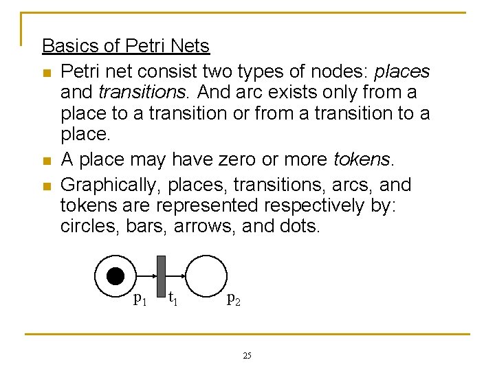
Basics of Petri Nets n Petri net consist two types of nodes: places and transitions. And arc exists only from a place to a transition or from a transition to a place. n A place may have zero or more tokens. n Graphically, places, transitions, arcs, and tokens are represented respectively by: circles, bars, arrows, and dots. p 1 t 1 p 2 25

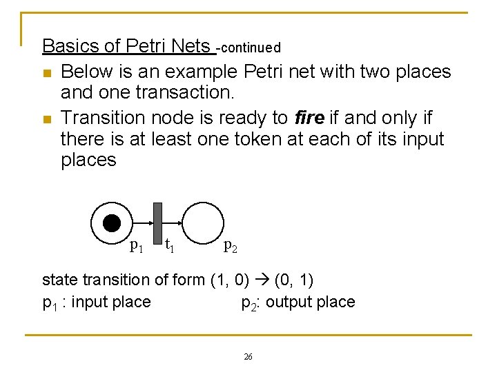
Basics of Petri Nets -continued n Below is an example Petri net with two places and one transaction. n Transition node is ready to fire if and only if there is at least one token at each of its input places p 1 t 1 p 2 state transition of form (1, 0) (0, 1) p 1 : input place p 2: output place 26

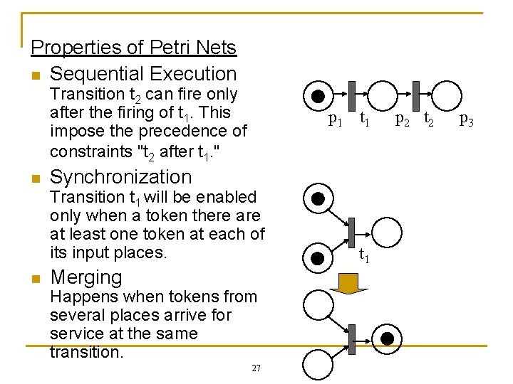
Properties of Petri Nets n Sequential Execution Transition t 2 can fire only after the firing of t 1. This impose the precedence of constraints "t 2 after t 1. " n p 1 t 1 Synchronization Transition t 1 will be enabled only when a token there at least one token at each of its input places. n Merging Happens when tokens from several places arrive for service at the same transition. 27 t 1 p 2 t 2 p 3

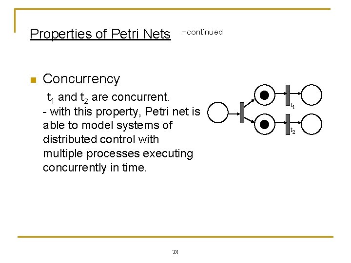
Properties of Petri Nets n -continued Concurrency t 1 and t 2 are concurrent. - with this property, Petri net is able to model systems of distributed control with multiple processes executing concurrently in time. 28 t 1 t 2

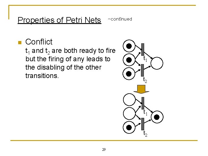
Properties of Petri Nets n -continued Conflict t 1 and t 2 are both ready to fire but the firing of any leads to the disabling of the other transitions. t 1 t 2 29

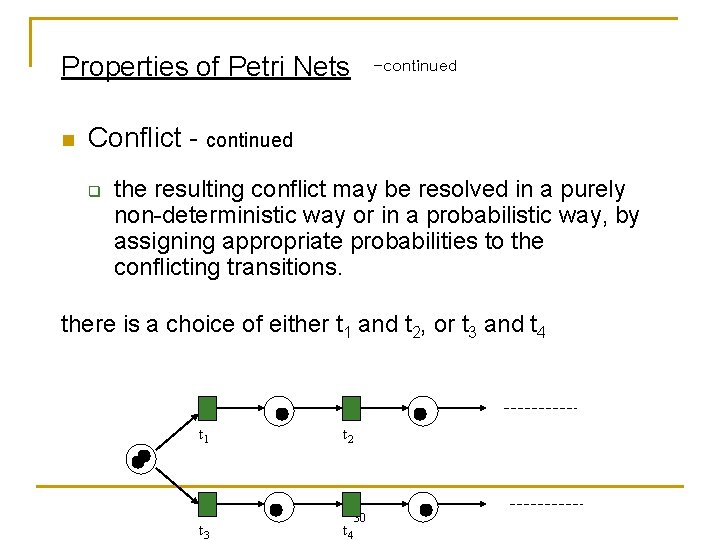
Properties of Petri Nets n -continued Conflict - continued q the resulting conflict may be resolved in a purely non-deterministic way or in a probabilistic way, by assigning appropriate probabilities to the conflicting transitions. there is a choice of either t 1 and t 2, or t 3 and t 4 t 1 t 2 t 3 t 4 30

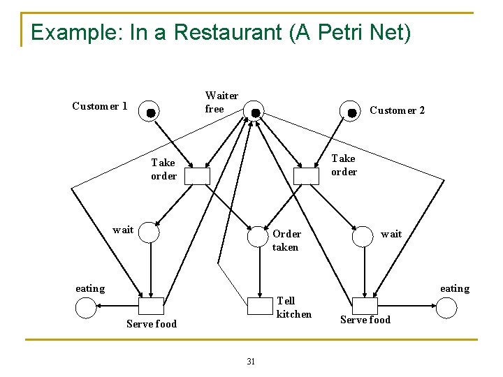
Example: In a Restaurant (A Petri Net) Waiter free Customer 1 Customer 2 Take order wait Order taken wait eating Tell kitchen Serve food 31 Serve food

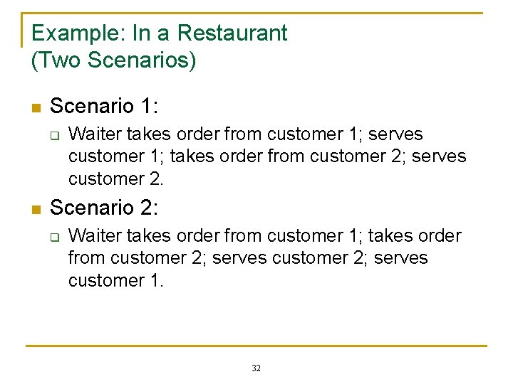
Example: In a Restaurant (Two Scenarios) n Scenario 1: q n Waiter takes order from customer 1; serves customer 1; takes order from customer 2; serves customer 2. Scenario 2: q Waiter takes order from customer 1; takes order from customer 2; serves customer 1. 32

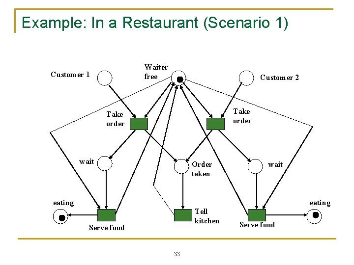
Example: In a Restaurant (Scenario 1) Waiter free Customer 1 Customer 2 Take order wait Order taken wait eating Tell kitchen Serve food 33 Serve food

Example: In a Restaurant (Scenario 2) Waiter free Customer 1 Customer 2 Take order wait Order taken wait eating Tell kitchen Serve food 34 Serve food

Petri Net with Time n n n 1962 - Carl Adam Petri originally proposed Petri without any notion of time. Concept of time was intentionally avoided because addition of time restricts the behavior of the net. 1970 s ~ - Addition of time has been discussed in order to analyze the performance of the modeled system. Many properties are still undecided for Petri nets extended with data and time. 35

References i Slides from lecture notes by q n www. cise. ufl. edu/~fishwick/cap 4800/pn 1. ppt For additional reading, refer to: q q http: //www. springerlink. com/content/978 -94 -007 -0257 -8#section=813480&page=1 Chapter : Specifications and Modeling , section 2. 6, page 67. You can read online using UCI internet access. 36

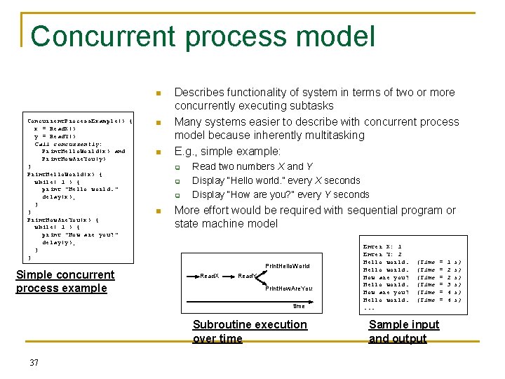
Concurrent process model n Concurrent. Process. Example() { x = Read. X() y = Read. Y() Call concurrently: Print. Hello. World(x) and Print. How. Are. You(y) } Print. Hello. World(x) { while( 1 ) { print "Hello world. " delay(x); } } Print. How. Are. You(x) { while( 1 ) { print "How are you? " delay(y); } } Simple concurrent process example n n Describes functionality of system in terms of two or more concurrently executing subtasks Many systems easier to describe with concurrent process model because inherently multitasking E. g. , simple example: q q q n Read two numbers X and Y Display “Hello world. ” every X seconds Display “How are you? ” every Y seconds More effort would be required with sequential program or state machine model Print. Hello. World Read. X Read. Y Print. How. Are. You time Subroutine execution over time 37 Enter X: 1 Enter Y: 2 Hello world. How are you? Hello world. . . . (Time (Time = = = Sample input and output 1 2 2 3 4 4 s) s) s)

Process Network n Task Graph (or process network) q Node: processes performing operations n n q Processes map intput data streams to output data streams Typical processes include iterations Edge: shows relation between the processes Winter 2010 - CS 244 38

Asynchronous message passing n n Communication between processes is buffered, typically assumed to be unbounded FIFOs. Kahn process network (KPN) q q n Writes are non-blocking, reads block when reading from empty FIFO. Only single process can read from FIFO. Synchronous data flow (SDF) Winter 2010 - CS 244 39

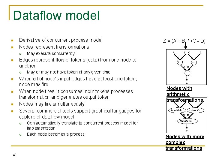
Dataflow model n n Derivative of concurrent process model Nodes represent transformations q n Edges represent flow of tokens (data) from one node to another q n n q A B C + Can automatically translate to concurrent process model for implementation Each node becomes a process D – t 1 t 2 May or may not have token at any given time When all of node’s input edges have at least one token, node may fire When node fires, it consumes input tokens processes transformation and generates output token Nodes may fire simultaneously Several commercial tools support graphical languages for capture of dataflow model q 40 May execute concurrently Z = (A + B) * (C - D) * Z Nodes with arithmetic transformations A B C D modulate convolve t 1 t 2 transform Z Nodes with more complex transformations

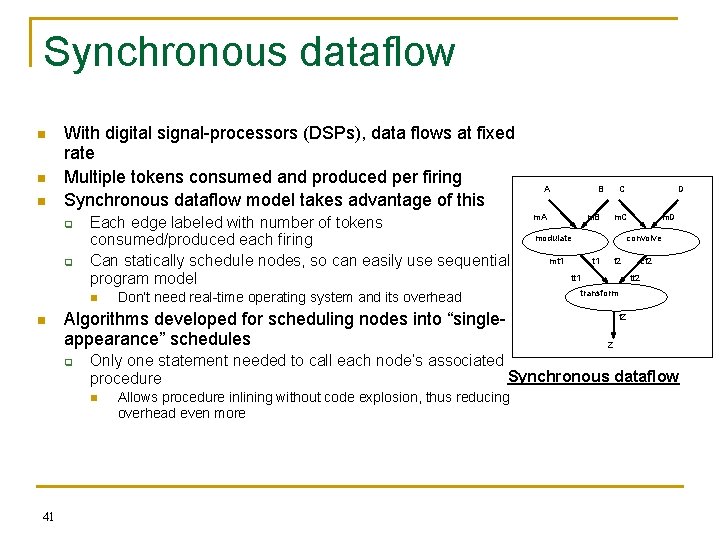
Synchronous dataflow n n n With digital signal-processors (DSPs), data flows at fixed rate Multiple tokens consumed and produced per firing Synchronous dataflow model takes advantage of this q q Each edge labeled with number of tokens consumed/produced each firing Can statically schedule nodes, so can easily use sequential program model n n Algorithms developed for scheduling nodes into “singleappearance” schedules q B m. A m. B C D m. C modulate m. D convolve mt 1 t 2 tt 1 ct 2 transform t. Z Z Only one statement needed to call each node’s associated Synchronous dataflow procedure n 41 Don’t need real-time operating system and its overhead A Allows procedure inlining without code explosion, thus reducing overhead even more