CS 240 A Computation on Graphs Graphs and

CS 240 A: Computation on Graphs

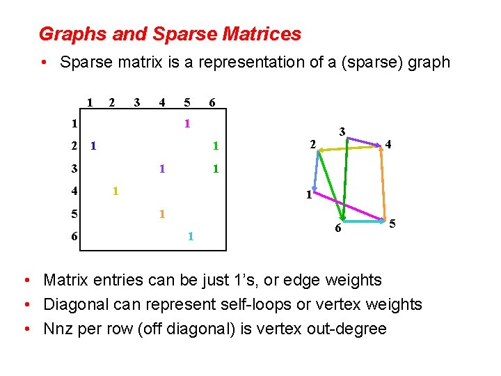
Graphs and Sparse Matrices • Sparse matrix is a representation of a (sparse) graph 1 2 3 4 1 1 2 1 5 6 6 1 1 3 4 5 1 1 4 1 1 1 2 3 1 1 6 5 • Matrix entries can be just 1’s, or edge weights • Diagonal can represent self-loops or vertex weights • Nnz per row (off diagonal) is vertex out-degree

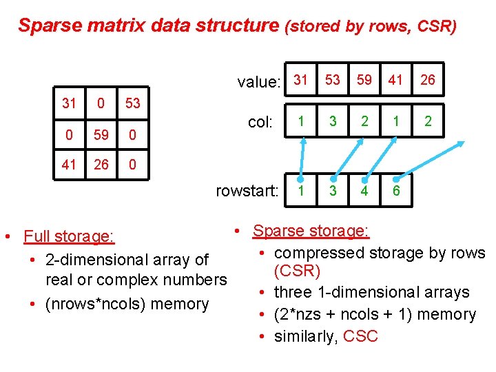
Sparse matrix data structure (stored by rows, CSR) value: 31 53 59 41 26 31 0 53 0 59 0 41 26 0 col: rowstart: 1 3 2 1 1 3 4 6 2 • Sparse storage: • Full storage: • compressed storage by rows • 2 -dimensional array of (CSR) real or complex numbers • three 1 -dimensional arrays • (nrows*ncols) memory • (2*nzs + ncols + 1) memory • similarly, CSC

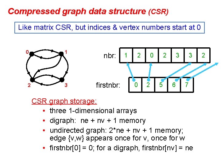
Compressed graph data structure (CSR) Like matrix CSR, but indices & vertex numbers start at 0 0 2 1 nbr: 3 firstnbr: 1 2 0 0 2 2 5 3 6 3 7 CSR graph storage: • three 1 -dimensional arrays • digraph: ne + nv + 1 memory • undirected graph: 2*ne + nv + 1 memory; edge {v, w} appears once for v, once for w • firstnbr[0] = 0; for a digraph, firstnbr[nv] = ne 2

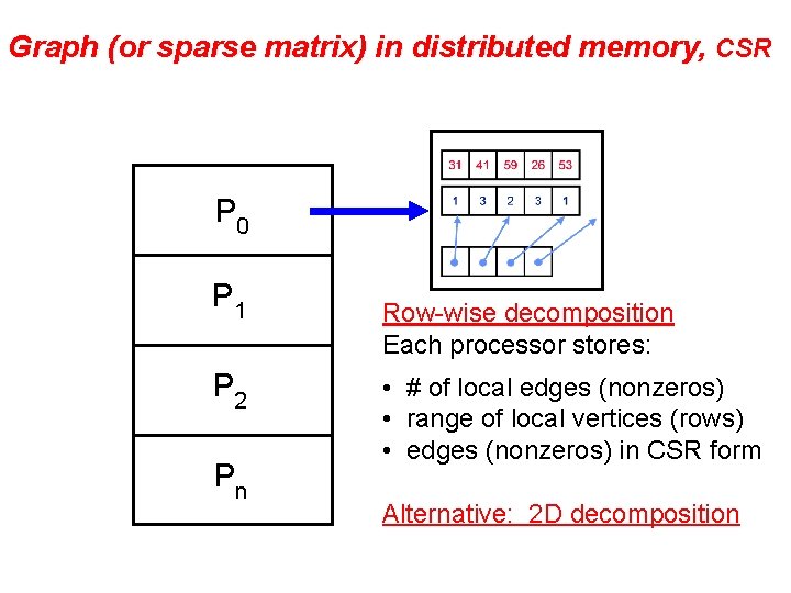
Graph (or sparse matrix) in distributed memory, CSR P 0 P 1 P 2 Pn Row-wise decomposition Each processor stores: • # of local edges (nonzeros) • range of local vertices (rows) • edges (nonzeros) in CSR form Alternative: 2 D decomposition

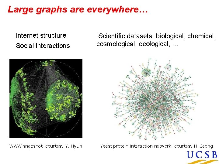
Large graphs are everywhere… Internet structure Social interactions WWW snapshot, courtesy Y. Hyun Scientific datasets: biological, chemical, cosmological, ecological, … Yeast protein interaction network, courtesy H. Jeong

Node-to-node searches in graphs … • • • Who are my friends’ friends? How many hops from A to B? (six degrees of Kevin Bacon) What’s the shortest route to Las Vegas? Am I related to Abraham Lincoln? Who likes the same movies I do, and what other movies do they like? • . . . • See breadth-first search example slides

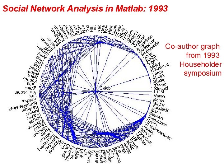
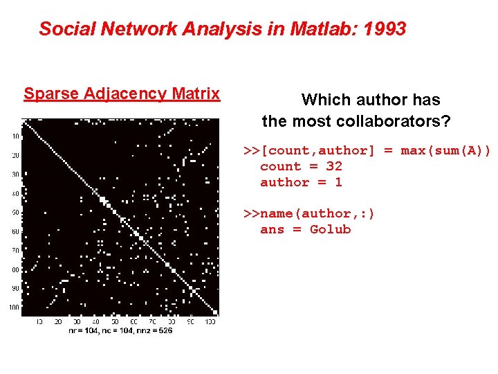
Social Network Analysis in Matlab: 1993 Co-author graph from 1993 Householder symposium

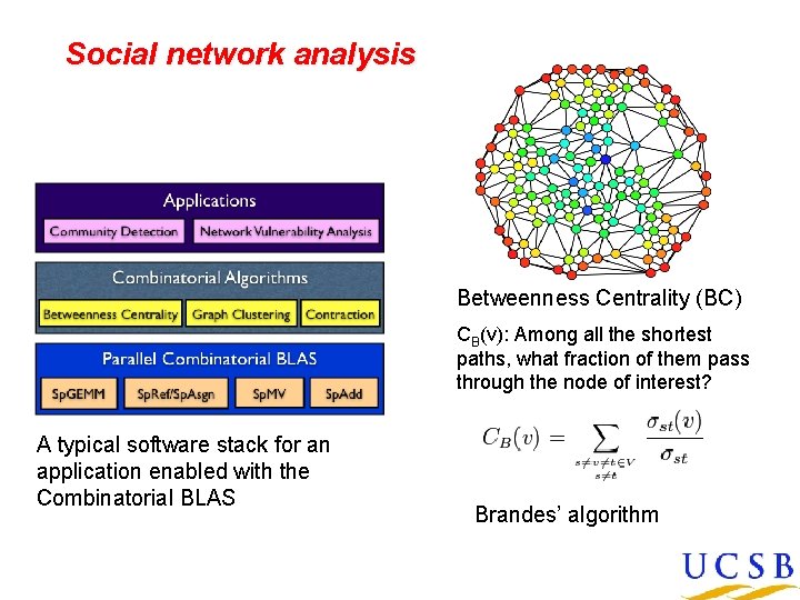
Social network analysis Betweenness Centrality (BC) CB(v): Among all the shortest paths, what fraction of them pass through the node of interest? A typical software stack for an application enabled with the Combinatorial BLAS Brandes’ algorithm

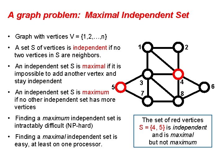
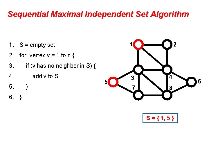
A graph problem: Maximal Independent Set • Graph with vertices V = {1, 2, …, n} • A set S of vertices is independent if no two vertices in S are neighbors. • An independent set S is maximal if it is impossible to add another vertex and stay independent 5 • An independent set S is maximum if no other independent set has more vertices • Finding a maximum independent set is intractably difficult (NP-hard) • Finding a maximal independent set is easy, at least on one processor. 1 2 3 4 7 8 The set of red vertices S = {4, 5} is independent and is maximal but not maximum 6

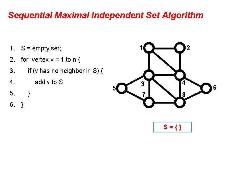
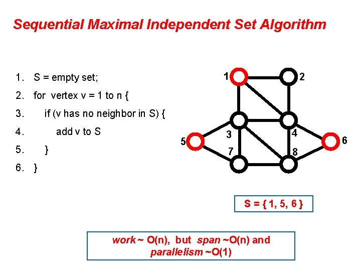
Sequential Maximal Independent Set Algorithm 1 1. S = empty set; 2 2. for vertex v = 1 to n { 3. if (v has no neighbor in S) { 4. 5. add v to S } 5 3 4 7 8 6. } S={} 6

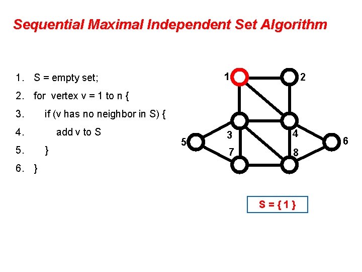
Sequential Maximal Independent Set Algorithm 1 1. S = empty set; 2 2. for vertex v = 1 to n { 3. if (v has no neighbor in S) { 4. 5. add v to S } 5 3 4 7 8 6. } S={1} 6

Sequential Maximal Independent Set Algorithm 1 1. S = empty set; 2 2. for vertex v = 1 to n { 3. if (v has no neighbor in S) { 4. 5. add v to S } 5 3 4 7 8 6. } S = { 1, 5 } 6

Sequential Maximal Independent Set Algorithm 1 1. S = empty set; 2 2. for vertex v = 1 to n { 3. if (v has no neighbor in S) { 4. 5. add v to S } 5 3 4 7 8 6. } S = { 1, 5, 6 } work ~ O(n), but span ~O(n) and parallelism ~O(1) 6

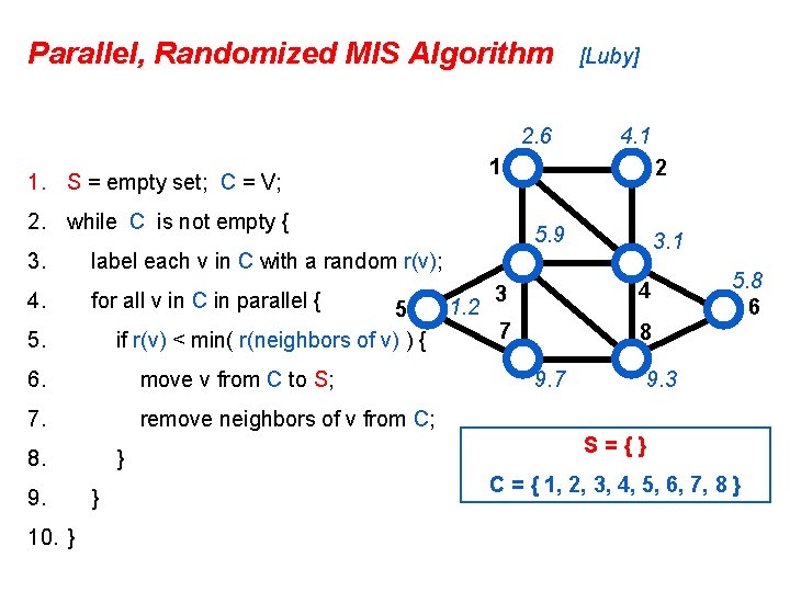
Parallel, Randomized MIS Algorithm 1. S = empty set; C = V; [Luby] 1 2 2. while C is not empty { 3. label each v in C with a random r(v); * 4. for all v in C in parallel { 5 if r(v) < min( r(neighbors of v) ) { 5. 6. move v from C to S; 7. remove neighbors of v from C; 8. 9. } } 10. } * (simplified version with some details omitted) 3 4 7 8 S={} C = { 1, 2, 3, 4, 5, 6, 7, 8 } 6

Parallel, Randomized MIS Algorithm 1. S = empty set; C = V; [Luby] 1 2 2. while C is not empty { 3. label each v in C with a random r(v); 4. for all v in C in parallel { 5 if r(v) < min( r(neighbors of v) ) { 5. 6. move v from C to S; 7. remove neighbors of v from C; 8. 9. 10. } } } 3 4 7 8 S={} C = { 1, 2, 3, 4, 5, 6, 7, 8 } 6

Parallel, Randomized MIS Algorithm 2. 6 2. while C is not empty { 4. for all v in C in parallel { 5 if r(v) < min( r(neighbors of v) ) { 6. move v from C to S; 7. remove neighbors of v from C; 8. 10. } 2 5. 9 3. 1 label each v in C with a random r(v); 5. 9. 4. 1 1 1. S = empty set; C = V; 3. [Luby] } } 1. 2 3 4 7 8 9. 7 5. 8 6 9. 3 S={} C = { 1, 2, 3, 4, 5, 6, 7, 8 }

Parallel, Randomized MIS Algorithm [Luby] 2. 6 1 1. S = empty set; C = V; 2. while C is not empty { 3. 4. for all v in C in parallel { 5 if r(v) < min( r(neighbors of v) ) { 6. move v from C to S; 7. remove neighbors of v from C; 8. 10. } 2 5. 9 3. 1 label each v in C with a random r(v); 5. 9. 4. 1 } } 1. 2 3 4 7 8 9. 7 9. 3 S = { 1, 5 } C = { 6, 8 } 5. 8 6

Parallel, Randomized MIS Algorithm 1. S = empty set; C = V; [Luby] 1 2 2. while C is not empty { 3. 4. label each v in C with a random r(v); for all v in C in parallel { 5 if r(v) < min( r(neighbors of v) ) { 5. 6. move v from C to S; 7. remove neighbors of v from C; 8. 9. 10. } } } 3 4 7 8 1. 8 S = { 1, 5 } C = { 6, 8 } 2. 7 6

Parallel, Randomized MIS Algorithm 1. S = empty set; C = V; [Luby] 1 2 2. while C is not empty { 3. 4. label each v in C with a random r(v); for all v in C in parallel { 5 if r(v) < min( r(neighbors of v) ) { 5. 6. move v from C to S; 7. remove neighbors of v from C; 8. 9. 10. } } } 3 4 7 8 1. 8 S = { 1, 5, 8 } C={} 2. 7 6

Parallel, Randomized MIS Algorithm 1. S = empty set; C = V; [Luby] 1 2 2. while C is not empty { 3. label each v in C with a random r(v); 4. for all v in C in parallel { 5 if r(v) < min( r(neighbors of v) ) { 5. 6. move v from C to S; 7. remove neighbors of v from C; 8. 9. 10. } } } 3 4 7 8 Theorem: This algorithm “very probably” finishes within O(log n) rounds. work ~ O(n log n), but span ~O(log 2 n), so parallelism ~O(n/log n) 6

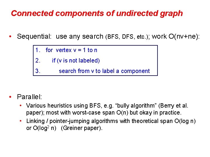
Connected components of undirected graph • Sequential: use any search (BFS, DFS, etc. ); work O(nv+ne): 1. for vertex v = 1 to n 2. 3. if (v is not labeled) search from v to label a component • Parallel: • Various heuristics using BFS, e. g. “bully algorithm” (Berry et al. paper); most with worst-case span O(n) but okay in practice. • Linking / pointer-jumping algorithms with theoretical span O(log n) or O(log 2 n) (Greiner paper).

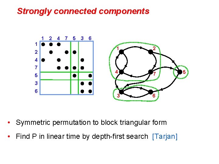
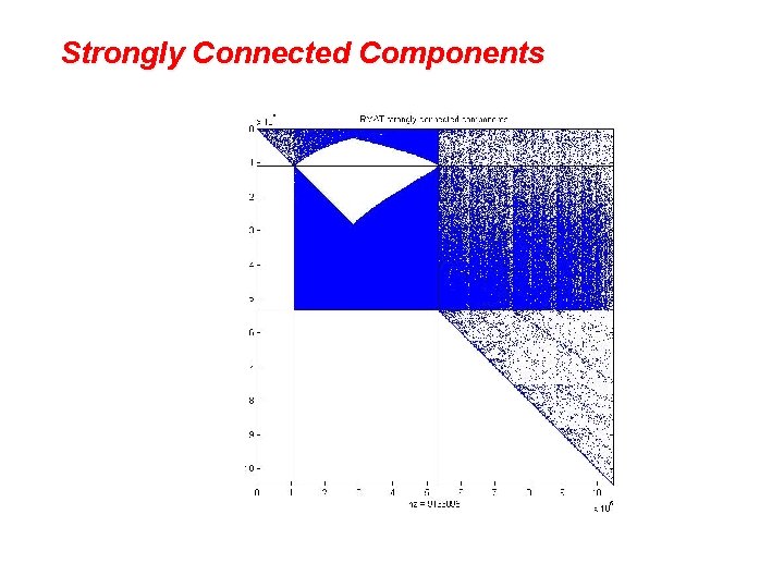
Strongly connected components 1 1 2 2 4 7 5 3 6 1 2 4 7 5 3 6 • Symmetric permutation to block triangular form • Find P in linear time by depth-first search [Tarjan] 5

Strongly Connected Components

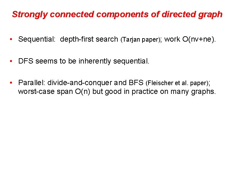
Strongly connected components of directed graph • Sequential: depth-first search (Tarjan paper); work O(nv+ne). • DFS seems to be inherently sequential. • Parallel: divide-and-conquer and BFS (Fleischer et al. paper); worst-case span O(n) but good in practice on many graphs.

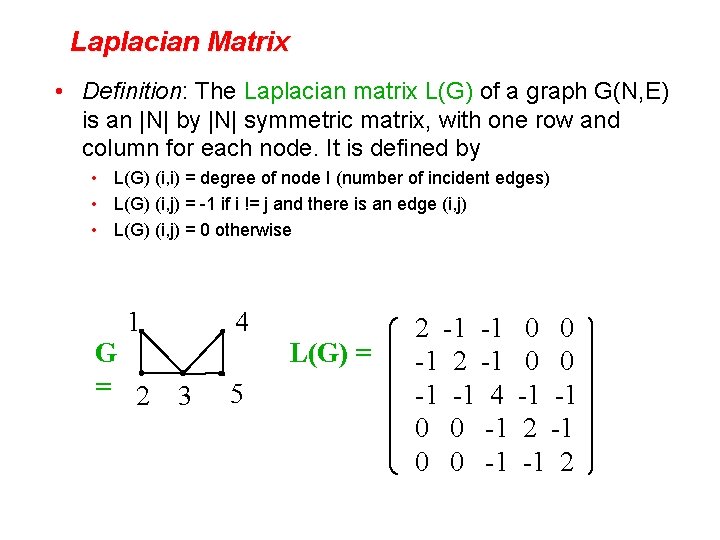
Laplacian Matrix • Definition: The Laplacian matrix L(G) of a graph G(N, E) is an |N| by |N| symmetric matrix, with one row and column for each node. It is defined by • L(G) (i, i) = degree of node I (number of incident edges) • L(G) (i, j) = -1 if i != j and there is an edge (i, j) • L(G) (i, j) = 0 otherwise 1 G = 2 3 4 L(G) = 5 2 -1 -1 -1 4 0 0 -1 -1 2

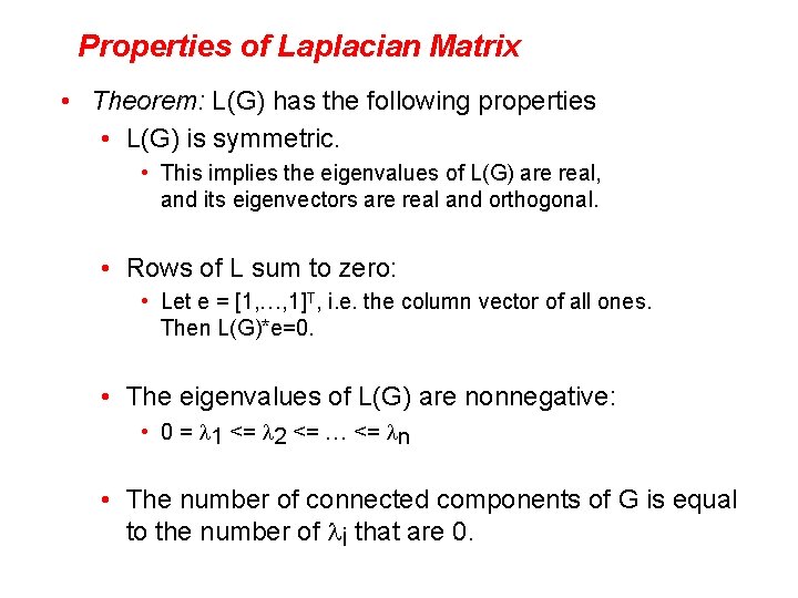
Properties of Laplacian Matrix • Theorem: L(G) has the following properties • L(G) is symmetric. • This implies the eigenvalues of L(G) are real, and its eigenvectors are real and orthogonal. • Rows of L sum to zero: • Let e = [1, …, 1]T, i. e. the column vector of all ones. Then L(G)*e=0. • The eigenvalues of L(G) are nonnegative: • 0 = l 1 <= l 2 <= … <= ln • The number of connected components of G is equal to the number of li that are 0.

EXTRA SLIDES

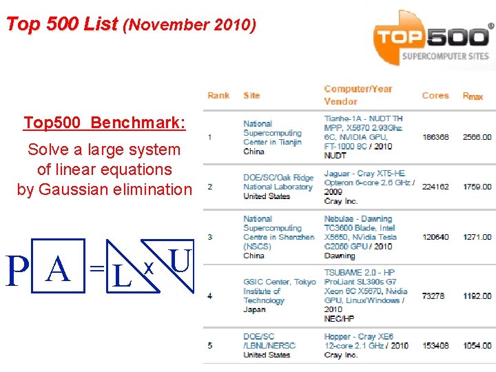
Top 500 List (November 2010) Top 500 Benchmark: Solve a large system of linear equations by Gaussian elimination P A = L x U

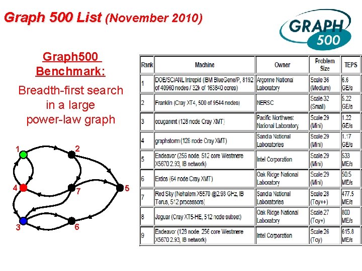
Graph 500 List (November 2010) Graph 500 Benchmark: Breadth-first search in a large power-law graph 1 2 4 7 3 6 5

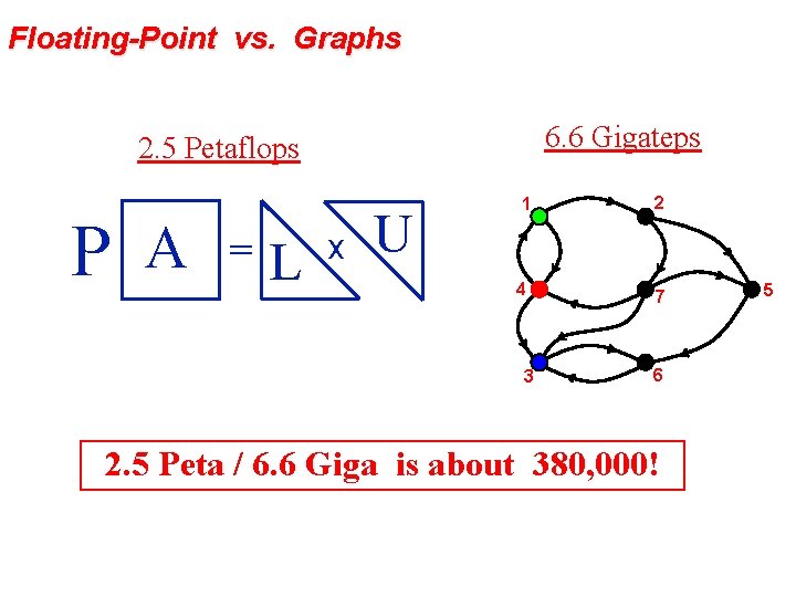
Floating-Point vs. Graphs 6. 6 Gigateps 2. 5 Petaflops P A = L x U 1 2 4 7 3 6 2. 5 Peta / 6. 6 Giga is about 380, 000! 5

Betweenness centrality • BC example from Robinson slides • BC sequential algorithm from Brandes paper • BC demo • Several potential sources of parallelism in BC

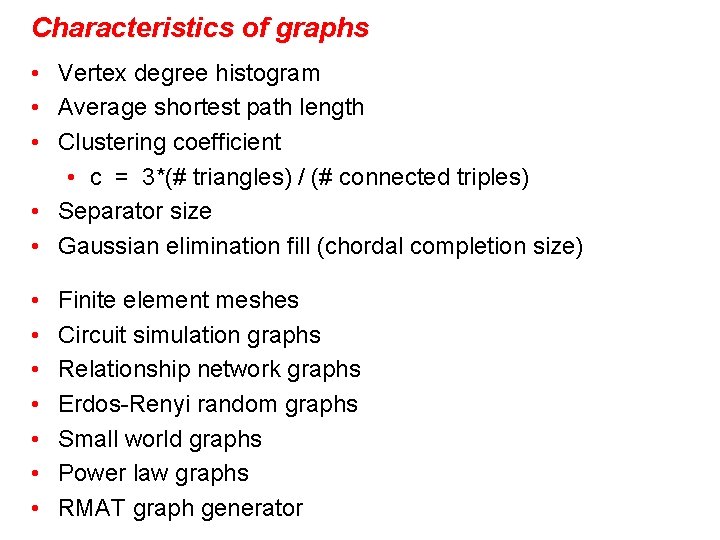
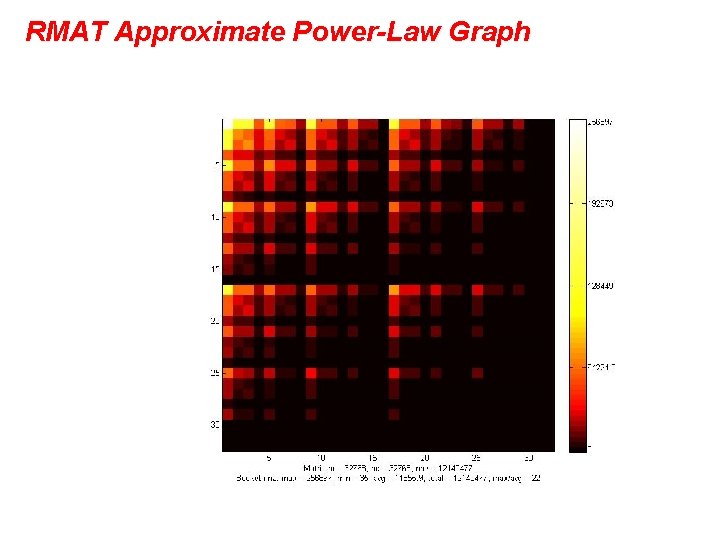
Characteristics of graphs • Vertex degree histogram • Average shortest path length • Clustering coefficient • c = 3*(# triangles) / (# connected triples) • Separator size • Gaussian elimination fill (chordal completion size) • • Finite element meshes Circuit simulation graphs Relationship network graphs Erdos-Renyi random graphs Small world graphs Power law graphs RMAT graph generator

RMAT Approximate Power-Law Graph

Strongly Connected Components

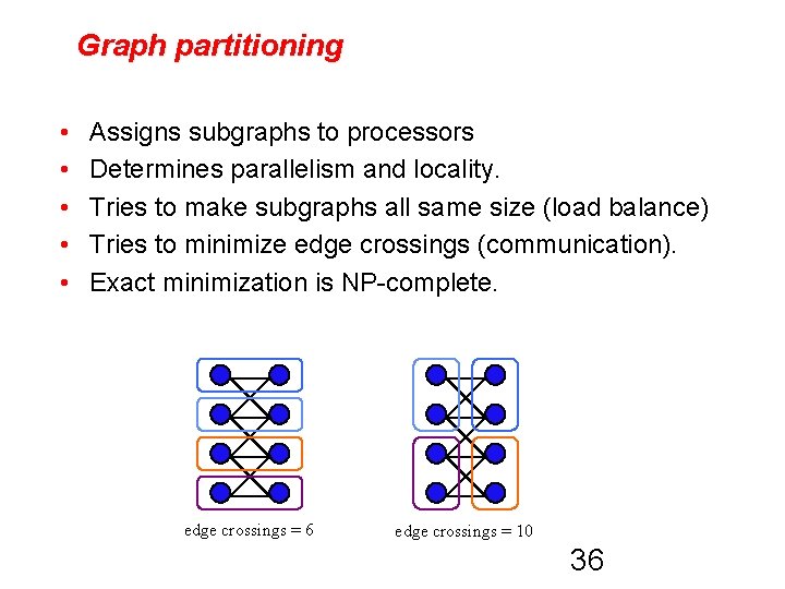
Graph partitioning • • • Assigns subgraphs to processors Determines parallelism and locality. Tries to make subgraphs all same size (load balance) Tries to minimize edge crossings (communication). Exact minimization is NP-complete. edge crossings = 6 edge crossings = 10 36

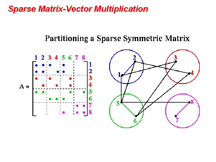
Sparse Matrix-Vector Multiplication

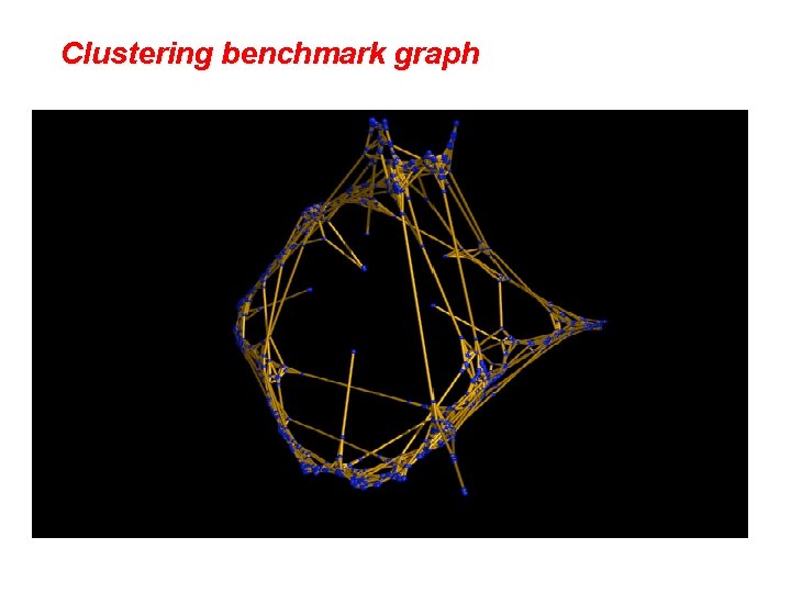
Clustering benchmark graph

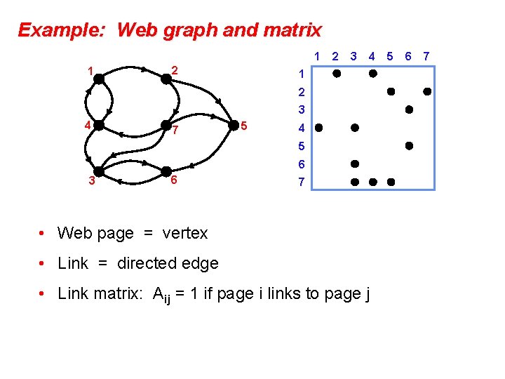
Example: Web graph and matrix 1 1 2 2 3 4 1 2 3 4 7 5 4 5 6 3 6 7 • Web page = vertex • Link = directed edge • Link matrix: Aij = 1 if page i links to page j 5 6 7

Web graph: Page. Rank (Google) [Brin, Page] An important page is one that many important pages point to. • Markov process: follow a random link most of the time; otherwise, go to any page at random. • Importance = stationary distribution of Markov process. • Transition matrix is p*A + (1 -p)*ones(size(A)), scaled so each column sums to 1. • Importance of page i is the i-th entry in the principal eigenvector of the transition matrix. • But the matrix is 1, 000, 000 by 1, 000, 000.

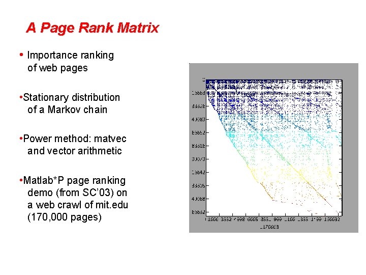
A Page Rank Matrix • Importance ranking of web pages • Stationary distribution of a Markov chain • Power method: matvec and vector arithmetic • Matlab*P page ranking demo (from SC’ 03) on a web crawl of mit. edu (170, 000 pages)

Social Network Analysis in Matlab: 1993 Co-author graph from 1993 Householder symposium

Social Network Analysis in Matlab: 1993 Sparse Adjacency Matrix Which author has the most collaborators? >>[count, author] = max(sum(A)) count = 32 author = 1 >>name(author, : ) ans = Golub

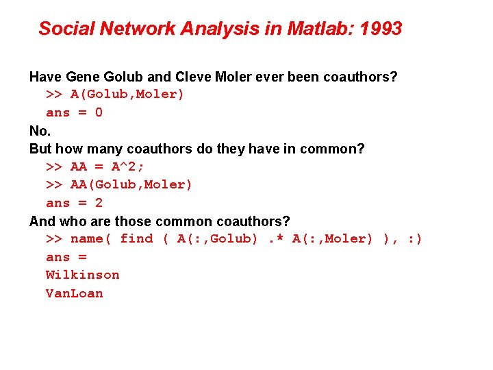
Social Network Analysis in Matlab: 1993 Have Gene Golub and Cleve Moler ever been coauthors? >> A(Golub, Moler) ans = 0 No. But how many coauthors do they have in common? >> AA = A^2; >> AA(Golub, Moler) ans = 2 And who are those common coauthors? >> name( find ( A(: , Golub). * A(: , Moler) ), : ) ans = Wilkinson Van. Loan

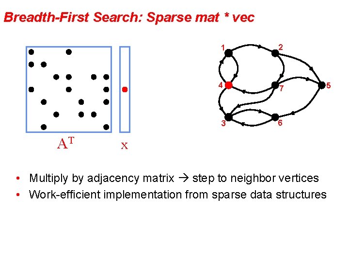
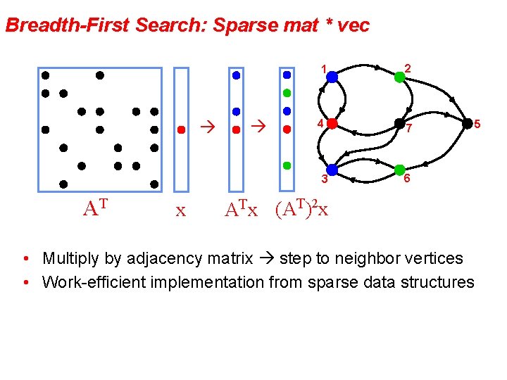
Breadth-First Search: Sparse mat * vec 1 2 4 7 3 AT x 6 AT x • Multiply by adjacency matrix step to neighbor vertices • Work-efficient implementation from sparse data structures 5

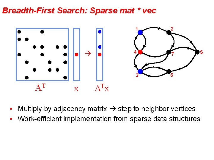
Breadth-First Search: Sparse mat * vec 1 2 4 7 3 AT x 6 AT x • Multiply by adjacency matrix step to neighbor vertices • Work-efficient implementation from sparse data structures 5

Breadth-First Search: Sparse mat * vec 1 2 4 7 3 AT x 6 ATx (AT)2 x • Multiply by adjacency matrix step to neighbor vertices • Work-efficient implementation from sparse data structures 5