CS 240 A Applied Parallel Computing Introduction 1

CS 240 A: Applied Parallel Computing Introduction 1

CS 240 A Course Information • Web page: http: //www. cs. ucsb. edu/~tyang/class/240 a 13 w • Class schedule: Mon/Wed. 11: 00 AM-12: 50 pm Phelp 2510 • Instructor: Tao Yang (tyang at cs). - Office Hours: MW 10 -11(or email me for appointments or just stop by my office). HFH building, Room 5113 • Supercomputing consultant: Kadir Diri and Stefan Boeriu • TA: - Wei Zhang (wei at cs). Office hours: Monday/Wed 3: 30 PM - 4: 30 PM • Class materials: - Slides/handouts. Research papers. Online references. • Slide source (HPC part) and related courses: - Demmel/Yelick's CS 267 parallel computing at UC Berkeley - John Gilbert‘s CS 240 A at UCSB 2

Topics • High performance computing - Basics of computer architecture, memory hierarchies, storage, clusters, cloud systems. - High throughput computing • Parallel Programming Models and Machines. Software/libraries - Shared memory vs distributed memory - Threads, Open. MP, MPI, Map. Reduce, GPU if time permits • Patterns of parallelism. Optimization techniques for parallelization and performance • Core algorithms in Scientific Computing and Applications - Dense & Sparse Linear Algebra • Parallelism in data-intensive web applications and storage systems 3

What you should get out of the course In depth understanding of: • When is parallel computing useful? • Understanding of parallel computing hardware options. • Overview of programming models (software) and tools. • Some important parallel applications and the algorithms • Performance analysis and tuning • Exposure to various open research questions 4

Introduction: Outline all • Why powerful computers must be parallel computing Including your laptops and handhelds • Why parallel processing? - Large Computational Science and Engineering (CSE) problems require powerful computers - Commercial data-oriented computing also needs. • Basic parallel performance models • Why writing (fast) parallel programs is hard 5

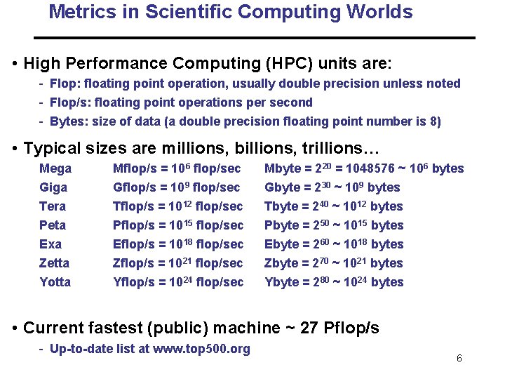
Metrics in Scientific Computing Worlds • High Performance Computing (HPC) units are: - Flop: floating point operation, usually double precision unless noted - Flop/s: floating point operations per second - Bytes: size of data (a double precision floating point number is 8) • Typical sizes are millions, billions, trillions… Mega Giga Tera Peta Exa Mflop/s = 106 flop/sec Gflop/s = 109 flop/sec Tflop/s = 1012 flop/sec Pflop/s = 1015 flop/sec Eflop/s = 1018 flop/sec Mbyte = 220 = 1048576 ~ 106 bytes Gbyte = 230 ~ 109 bytes Tbyte = 240 ~ 1012 bytes Pbyte = 250 ~ 1015 bytes Ebyte = 260 ~ 1018 bytes Zetta Zflop/s = 1021 flop/sec Zbyte = 270 ~ 1021 bytes Yotta Yflop/s = 1024 flop/sec Ybyte = 280 ~ 1024 bytes • Current fastest (public) machine ~ 27 Pflop/s - Up-to-date list at www. top 500. org 6

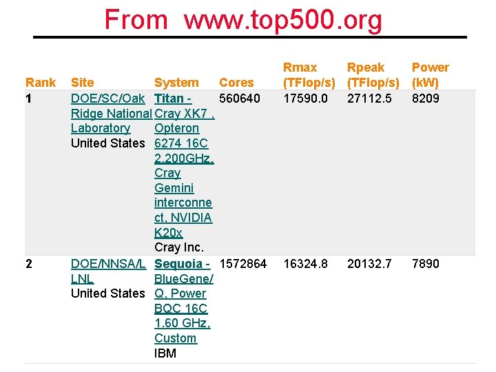
From www. top 500. org Rank 1 2 Site System Cores DOE/SC/Oak Titan - 560640 Ridge National Cray XK 7 , Laboratory Opteron United States 6274 16 C 2. 200 GHz, Cray Gemini interconne ct, NVIDIA K 20 x Cray Inc. DOE/NNSA/L Sequoia - 1572864 LNL Blue. Gene/ United States Q, Power BQC 16 C 1. 60 GHz, Custom IBM Rmax Rpeak Power (TFlop/s) (k. W) 17590. 0 27112. 5 8209 16324. 8 20132. 7 7890

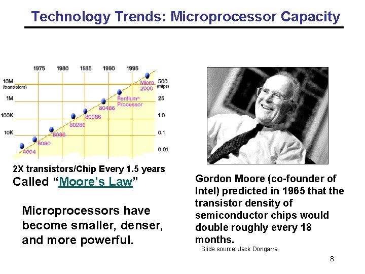
Technology Trends: Microprocessor Capacity Moore’s Law 2 X transistors/Chip Every 1. 5 years Called “Moore’s Law” Microprocessors have become smaller, denser, and more powerful. Gordon Moore (co-founder of Intel) predicted in 1965 that the transistor density of semiconductor chips would double roughly every 18 months. Slide source: Jack Dongarra 8

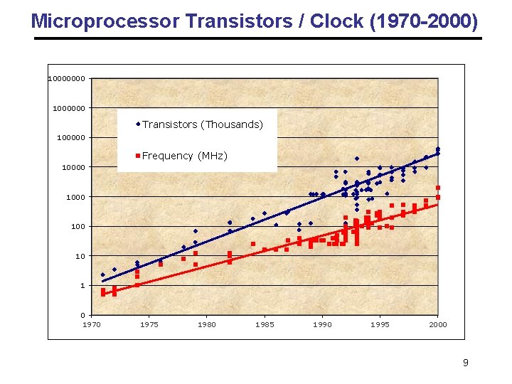
Microprocessor Transistors / Clock (1970 -2000) 10000000 1000000 Transistors (Thousands) 100000 Frequency (MHz) 10000 100 10 1 0 1975 1980 1985 1990 1995 2000 9

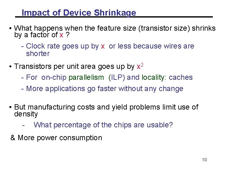
Impact of Device Shrinkage • What happens when the feature size (transistor size) shrinks by a factor of x ? - Clock rate goes up by x or less because wires are shorter • Transistors per unit area goes up by x 2 - For on-chip parallelism (ILP) and locality: caches - More applications go faster without any change • But manufacturing costs and yield problems limit use of density - What percentage of the chips are usable? & More power consumption 10

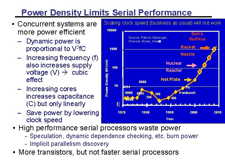
Power Density Limits Serial Performance – Dynamic power is proportional to V 2 f. C – Increasing frequency (f) also increases supply voltage (V) cubic effect – Increasing cores increases capacitance (C) but only linearly – Save power by lowering clock speed Scaling clock speed (business as usual) will not work 10000 Sun’s Surface Source: Patrick Gelsinger, Shenkar Bokar, Intel Rocket 1000 Nozzle Power Density (W/cm 2) • Concurrent systems are more power efficient Nuclear 100 Reactor Hot Plate 8086 10 4004 8008 8080 P 6 8085 286 Pentium® 386 486 1 1970 1980 1990 2000 Year • High performance serial processors waste power - Speculation, dynamic dependence checking, etc. burn power - Implicit parallelism discovery • More transistors, but not faster serial processors 2010

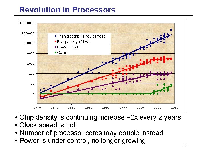
Revolution in Processors 10000000 1000000 100000 10000 Transistors (Thousands) Frequency (MHz) Power Cores (W) Cores 1000 100 10 10 1 1 0 1970 • • 1975 1980 1985 1990 1995 2000 2005 2010 Chip density is continuing increase ~2 x every 2 years Clock speed is not Number of processor cores may double instead Power is under control, no longer growing 12

Impact of Parallelism • All major processor vendors are producing multicore chips - Every machine will soon be a parallel machine - To keep doubling performance, parallelism must double • Which commercial applications can use this parallelism? - Do they have to be rewritten from scratch? • Will all programmers have to be parallel programmers? - New software model needed - Try to hide complexity from most programmers – eventually • Computer industry betting on this big change, but does not have all the answers 13

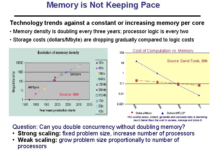
Memory is Not Keeping Pace Technology trends against a constant or increasing memory per core • Memory density is doubling every three years; processor logic is every two • Storage costs (dollars/Mbyte) are dropping gradually compared to logic costs Cost of Computation vs. Memory Source: David Turek, IBM Source: IBM Question: Can you double concurrency without doubling memory? • Strong scaling: fixed problem size, increase number of processors • Weak scaling: grow problem size proportionally to number of processors

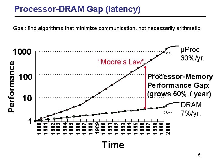
Processor-DRAM Gap (latency) Goal: find algorithms that minimize communication, not necessarily arithmetic CPU “Moore’s Law” 100 Processor-Memory Performance Gap: (grows 50% / year) DRAM 7%/yr. 10 1 µProc 60%/yr. 1980 1981 1982 1983 1984 1985 1986 1987 1988 1989 1990 1991 1992 1993 1994 1995 1996 1997 1998 1999 2000 Performance 1000 Time 15

The TOP 500 Project • Listing the 500 most powerful computers in the world • Linpack performance - Solve Ax=b, dense problem, matrix is random - Dominated by dense matrix-matrix multiply • Update twice a year: - ISC’xy in June in Germany - SCxy in November in the U. S. • All information available from the TOP 500 web site at: www. top 500. org

Moore’s Law reinterpreted • Number of cores per chip will double every two years • Clock speed will not increase (possibly decrease) • Need to deal with systems with millions of concurrent threads • Need to deal with inter-chip parallelism as well as intra-chip parallelism

Outline all • Why powerful computers must be parallel processors Including your laptops and handhelds • Large Computational Science&Engineering and commercial problems require powerful computers • Basic performance models • Why writing (fast) parallel programs is hard 18

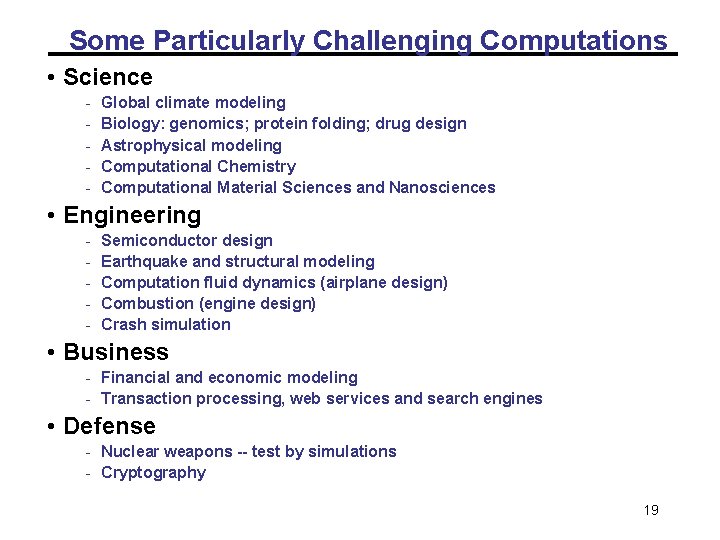
Some Particularly Challenging Computations • Science - Global climate modeling Biology: genomics; protein folding; drug design Astrophysical modeling Computational Chemistry Computational Material Sciences and Nanosciences • Engineering - Semiconductor design Earthquake and structural modeling Computation fluid dynamics (airplane design) Combustion (engine design) Crash simulation • Business - Financial and economic modeling - Transaction processing, web services and search engines • Defense - Nuclear weapons -- test by simulations - Cryptography 19

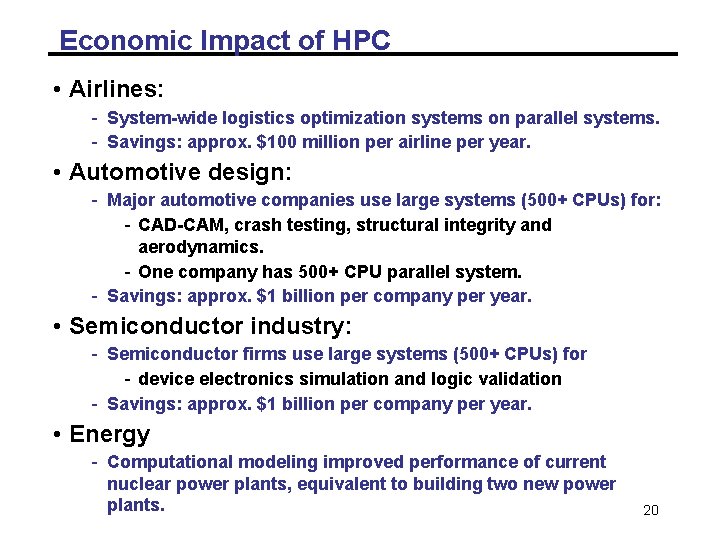
Economic Impact of HPC • Airlines: - System-wide logistics optimization systems on parallel systems. - Savings: approx. $100 million per airline per year. • Automotive design: - Major automotive companies use large systems (500+ CPUs) for: - CAD-CAM, crash testing, structural integrity and aerodynamics. - One company has 500+ CPU parallel system. - Savings: approx. $1 billion per company per year. • Semiconductor industry: - Semiconductor firms use large systems (500+ CPUs) for - device electronics simulation and logic validation - Savings: approx. $1 billion per company per year. • Energy - Computational modeling improved performance of current nuclear power plants, equivalent to building two new power plants. 20

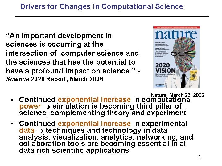
Drivers for Changes in Computational Science “An important development in sciences is occurring at the intersection of computer science and the sciences that has the potential to have a profound impact on science. ” Science 2020 Report, March 2006 Nature, March 23, 2006 • Continued exponential increase in computational power simulation is becoming third pillar of science, complementing theory and experiment • Continued exponential increase in experimental data techniques and technology in data analysis, visualization, analytics, networking, and collaboration tools are becoming essential in all data rich scientific applications 21

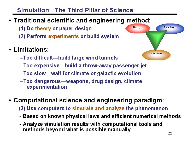
Simulation: The Third Pillar of Science • Traditional scientific and engineering method: (1) Do theory or paper design (2) Perform experiments or build system Theory • Limitations: –Too difficult—build large wind tunnels Experiment Simulation –Too expensive—build a throw-away passenger jet –Too slow—wait for climate or galactic evolution –Too dangerous—weapons, drug design, climate experimentation • Computational science and engineering paradigm: (3) Use computers to simulate and analyze the phenomenon - Based on known physical laws and efficient numerical methods - Analyze simulation results with computational tools and methods beyond what is possible manually 22

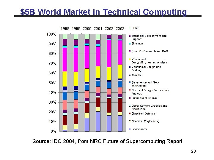
$5 B World Market in Technical Computing Source: IDC 2004, from NRC Future of Supercomputing Report 23

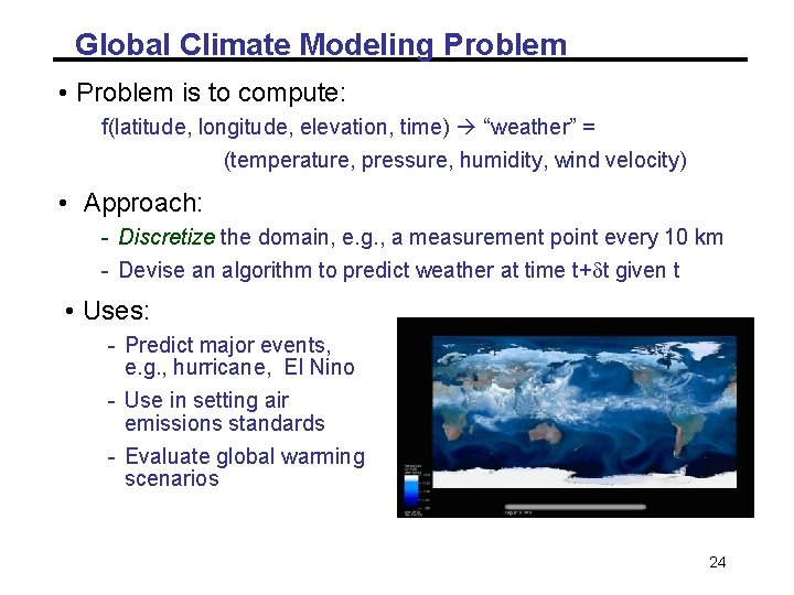
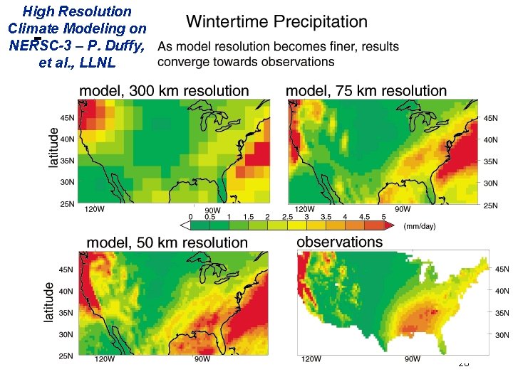
Global Climate Modeling Problem • Problem is to compute: f(latitude, longitude, elevation, time) “weather” = (temperature, pressure, humidity, wind velocity) • Approach: - Discretize the domain, e. g. , a measurement point every 10 km - Devise an algorithm to predict weather at time t+dt given t • Uses: - Predict major events, e. g. , hurricane, El Nino - Use in setting air emissions standards - Evaluate global warming scenarios 24

Global Climate Modeling Computation • One piece is modeling the fluid flow in the atmosphere - Solve Navier-Stokes equations - Roughly 100 Flops per grid point with 1 minute timestep • Computational requirements: - To match real-time, need 5 x 1011 flops in 60 seconds = 8 Gflop/s Weather prediction (7 days in 24 hours) 56 Gflop/s Climate prediction (50 years in 30 days) 4. 8 Tflop/s To use in policy negotiations (50 years in 12 hours) 288 Tflop/s • To double the grid resolution, computation is 8 x to 16 x • State of the art models require integration of atmosphere, clouds, ocean, sea-ice, land models, plus possibly carbon cycle, geochemistry and more • Current models are coarser than this 25

High Resolution Climate Modeling on NERSC-3 – P. Duffy, et al. , LLNL 26

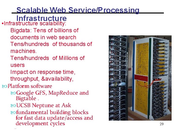
Scalable Web Service/Processing Infrastructure • Infrastructure scalability: Bigdata: Tens of billions of documents in web search Tens/hundreds of thousands of machines. Tens/hundreds of Millions of users Impact on response time, throughput, &availability, Platform software Google GFS, Map. Reduce and Bigtable. UCSB Neptune at Ask fundamental building blocks for fast data update/access and development cycles … 29

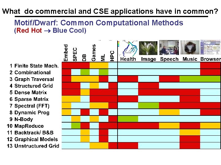
What do commercial and CSE applications have in common? Motif/Dwarf: Common Computational Methods (Red Hot Blue Cool)

Outline all • Why powerful computers must be parallel processors Including your laptops and handhelds • Large CSE problems require powerful computers Commercial problems too • Basic parallel performance models • Why writing (fast) parallel programs is hard 31

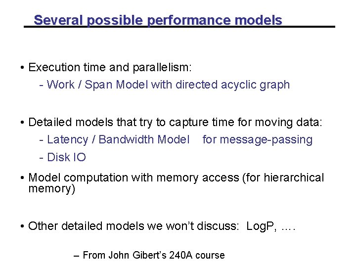
Several possible performance models • Execution time and parallelism: - Work / Span Model with directed acyclic graph • Detailed models that try to capture time for moving data: - Latency / Bandwidth Model for message-passing - Disk IO • Model computation with memory access (for hierarchical memory) • Other detailed models we won’t discuss: Log. P, …. – From John Gibert’s 240 A course

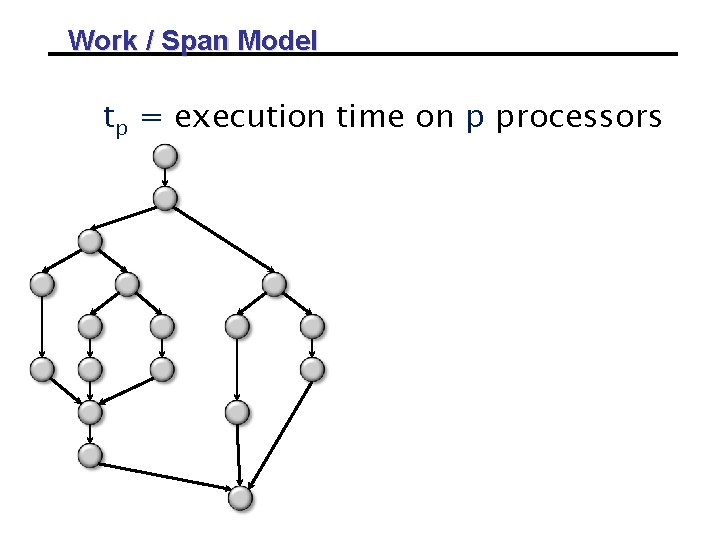
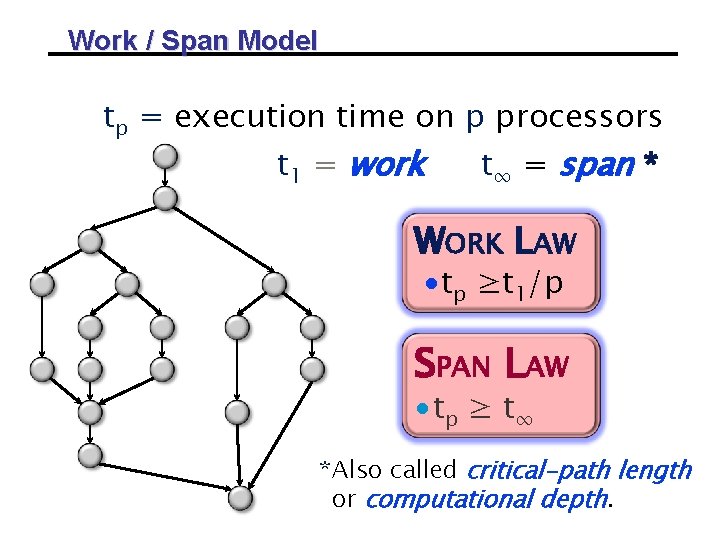
Work / Span Model tp = execution time on p processors

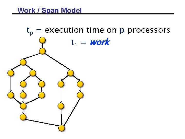
Work / Span Model tp = execution time on p processors t 1 = work

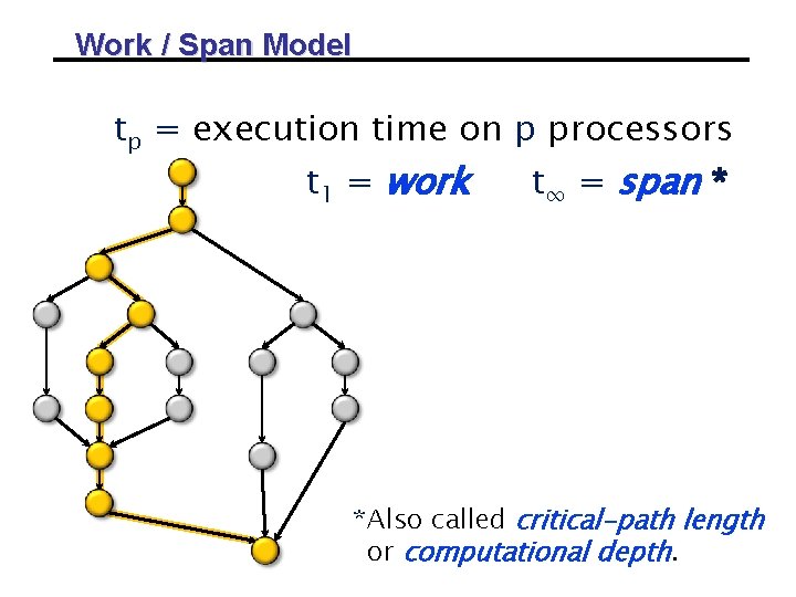
Work / Span Model tp = execution time on p processors t 1 = work t∞ = span * *Also called critical-path length or computational depth.

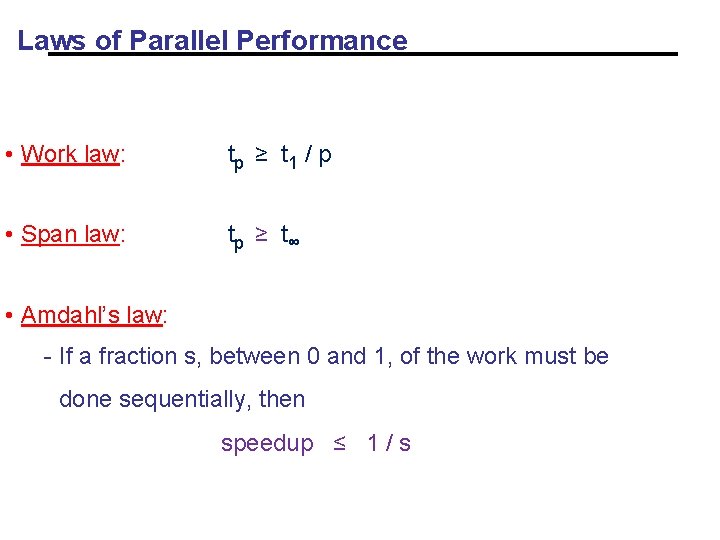
Work / Span Model tp = execution time on p processors t 1 = work t∞ = span * WORK LAW ∙tp ≥t 1/p SPAN LAW ∙ tp ≥ t ∞ *Also called critical-path length or computational depth.

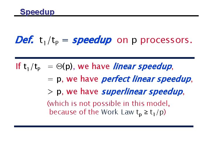
Speedup Def. t 1/t. P = speedup on p processors. If t 1/t. P = (p), we have linear speedup, = p, we have perfect linear speedup, > p, we have superlinear speedup, (which is not possible in this model, because of the Work Law tp ≥ t 1/p)

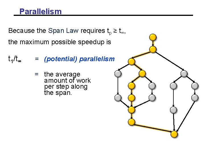
Parallelism Because the Span Law requires tp ≥ t∞, the maximum possible speedup is t 1/t∞ = (potential) parallelism = the average amount of work per step along the span.

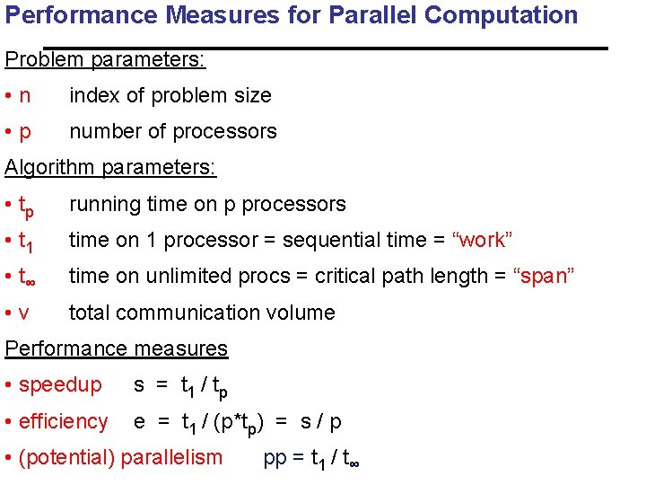
Performance Measures for Parallel Computation Problem parameters: • n index of problem size • p number of processors Algorithm parameters: • tp running time on p processors • t 1 time on 1 processor = sequential time = “work” • t∞ time on unlimited procs = critical path length = “span” • v total communication volume Performance measures • speedup s = t 1 / tp • efficiency e = t 1 / (p*tp) = s / p • (potential) parallelism pp = t 1 / t∞

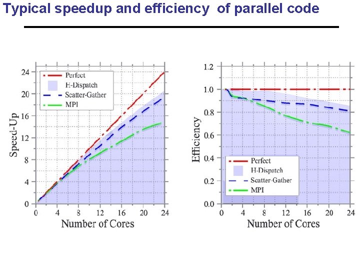
Typical speedup and efficiency of parallel code

Laws of Parallel Performance • Work law: tp ≥ t 1 / p • Span law: tp ≥ t∞ • Amdahl’s law: - If a fraction s, between 0 and 1, of the work must be done sequentially, then speedup ≤ 1 / s

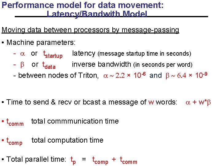
Performance model for data movement: Latency/Bandwith Model Moving data between processors by message-passing • Machine parameters: - a or tstartup latency (message startup time in seconds) - b or tdata inverse bandwidth (in seconds per word) - between nodes of Triton, a ~ 2. 2 × 10 -6 and b ~ 6. 4 × 10 -9 • Time to send & recv or bcast a message of w words: a + w*b • tcomm total commmunication time • tcomp total computation time • Total parallel time: tp = tcomp + tcomm

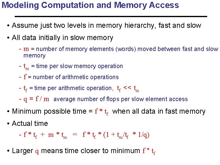
Modeling Computation and Memory Access • Assume just two levels in memory hierarchy, fast and slow • All data initially in slow memory - m = number of memory elements (words) moved between fast and slow memory - tm = time per slow memory operation - f = number of arithmetic operations - tf = time per arithmetic operation, tf << tm - q = f / m average number of flops per slow element access • Minimum possible time = f * tf when all data in fast memory • Actual time - f * tf + m * tm = f * tf * (1 + tm/tf * 1/q) • Larger q means time closer to minimum f * tf

Outline all • Why powerful computers must be parallel processors Including your laptops and handhelds • Large CSE/commerical problems require powerful computers • Performance models • Why writing (fast) parallel programs is hard 44

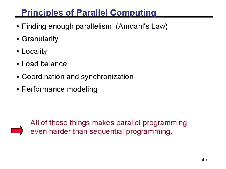
Principles of Parallel Computing • Finding enough parallelism (Amdahl’s Law) • Granularity • Locality • Load balance • Coordination and synchronization • Performance modeling All of these things makes parallel programming even harder than sequential programming. 45

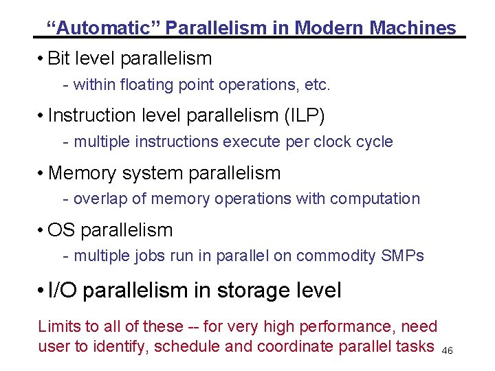
“Automatic” Parallelism in Modern Machines • Bit level parallelism - within floating point operations, etc. • Instruction level parallelism (ILP) - multiple instructions execute per clock cycle • Memory system parallelism - overlap of memory operations with computation • OS parallelism - multiple jobs run in parallel on commodity SMPs • I/O parallelism in storage level Limits to all of these -- for very high performance, need user to identify, schedule and coordinate parallel tasks 46

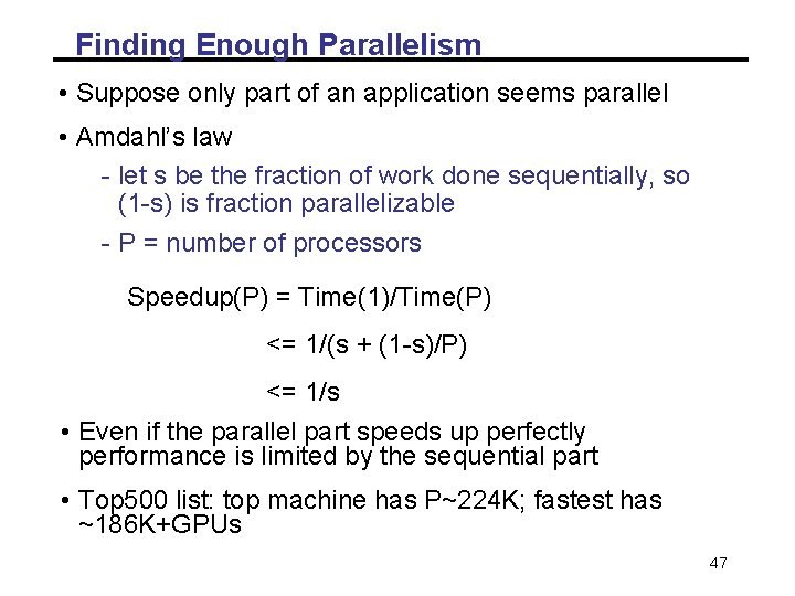
Finding Enough Parallelism • Suppose only part of an application seems parallel • Amdahl’s law - let s be the fraction of work done sequentially, so (1 -s) is fraction parallelizable - P = number of processors Speedup(P) = Time(1)/Time(P) <= 1/(s + (1 -s)/P) <= 1/s • Even if the parallel part speeds up perfectly performance is limited by the sequential part • Top 500 list: top machine has P~224 K; fastest has ~186 K+GPUs 47

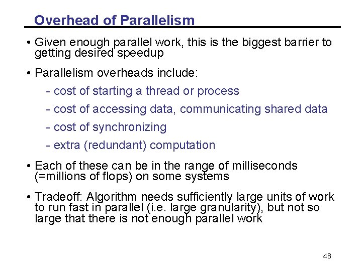
Overhead of Parallelism • Given enough parallel work, this is the biggest barrier to getting desired speedup • Parallelism overheads include: - cost of starting a thread or process - cost of accessing data, communicating shared data - cost of synchronizing - extra (redundant) computation • Each of these can be in the range of milliseconds (=millions of flops) on some systems • Tradeoff: Algorithm needs sufficiently large units of work to run fast in parallel (i. e. large granularity), but not so large that there is not enough parallel work 48

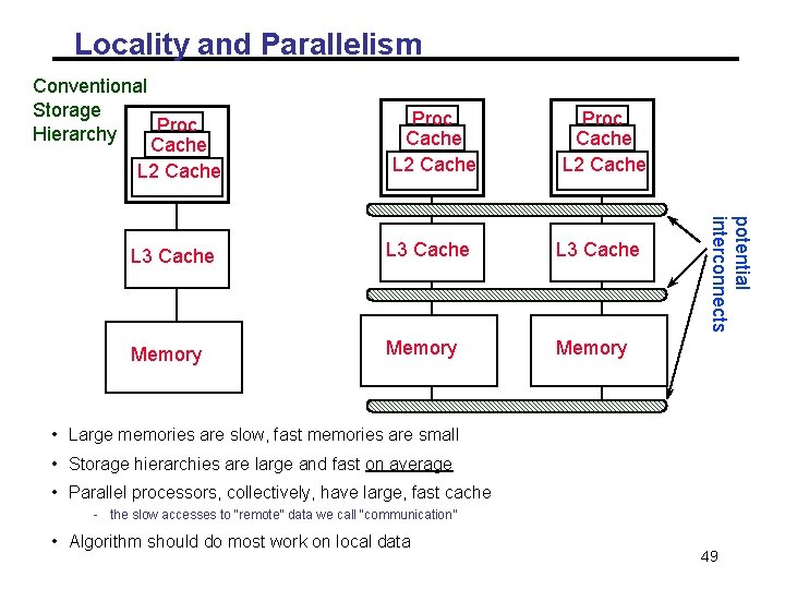
Locality and Parallelism Conventional Storage Proc Hierarchy Cache L 2 Cache Proc Cache L 2 Cache L 3 Cache Memory potential interconnects L 3 Cache • Large memories are slow, fast memories are small • Storage hierarchies are large and fast on average • Parallel processors, collectively, have large, fast cache - the slow accesses to “remote” data we call “communication” • Algorithm should do most work on local data 49

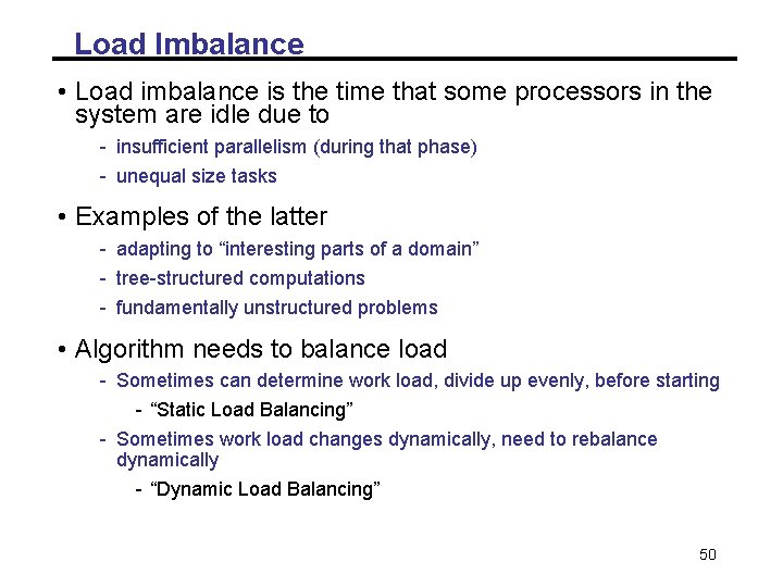
Load Imbalance • Load imbalance is the time that some processors in the system are idle due to - insufficient parallelism (during that phase) - unequal size tasks • Examples of the latter - adapting to “interesting parts of a domain” - tree-structured computations - fundamentally unstructured problems • Algorithm needs to balance load - Sometimes can determine work load, divide up evenly, before starting - “Static Load Balancing” - Sometimes work load changes dynamically, need to rebalance dynamically - “Dynamic Load Balancing” 50

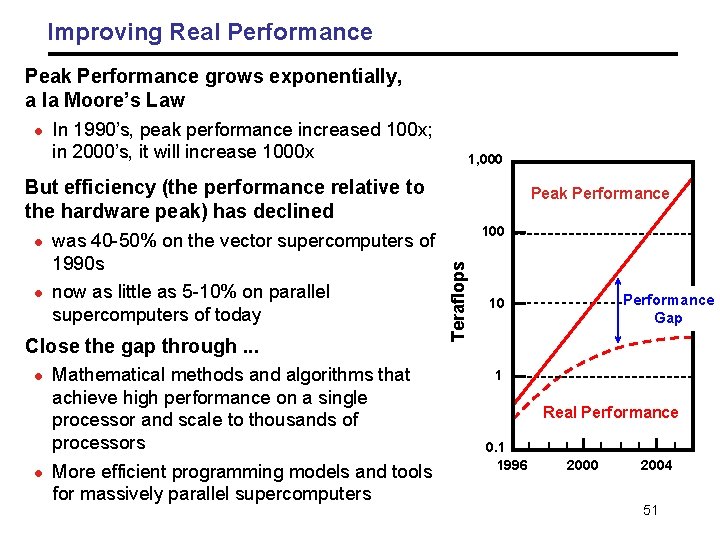
Improving Real Performance Peak Performance grows exponentially, a la Moore’s Law l In 1990’s, peak performance increased 100 x; in 2000’s, it will increase 1000 x 1, 000 But efficiency (the performance relative to the hardware peak) has declined l was 40 -50% on the vector supercomputers of 1990 s now as little as 5 -10% on parallel supercomputers of today Close the gap through. . . l l Mathematical methods and algorithms that achieve high performance on a single processor and scale to thousands of processors More efficient programming models and tools for massively parallel supercomputers 100 Teraflops l Peak Performance Gap 10 1 Real Performance 0. 1 1996 2000 2004 51

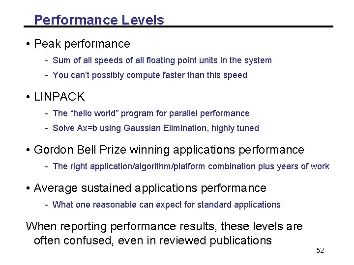
Performance Levels • Peak performance - Sum of all speeds of all floating point units in the system - You can’t possibly compute faster than this speed • LINPACK - The “hello world” program for parallel performance - Solve Ax=b using Gaussian Elimination, highly tuned • Gordon Bell Prize winning applications performance - The right application/algorithm/platform combination plus years of work • Average sustained applications performance - What one reasonable can expect for standard applications When reporting performance results, these levels are often confused, even in reviewed publications 52

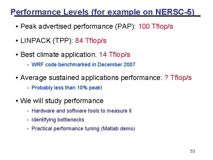
Performance Levels (for example on NERSC-5) • Peak advertised performance (PAP): 100 Tflop/s • LINPACK (TPP): 84 Tflop/s • Best climate application: 14 Tflop/s - WRF code benchmarked in December 2007 • Average sustained applications performance: ? Tflop/s - Probably less than 10% peak! • We will study performance - Hardware and software tools to measure it - Identifying bottlenecks - Practical performance tuning (Matlab demo) 53

What you should get out of the course In depth understanding of: • When is parallel computing useful? • Understanding of parallel computing hardware options. • Overview of programming models (software) and tools. • Some important parallel applications and the algorithms • Performance analysis and tuning • Exposure to various open research questions 54

Course Deadlines (Tentative) • Week 1: join Google discussion group. Email your name, UCSB email, and ssh key to scc@oit. ucsb. edu for Triton account. • Jan 27: 1 -page project proposal. The content includes: Problem description, challenges (what is new? ), what to deliver, how to test and what to measure, milestones, and references • Jan 29 week: Meet with me on the proposal and paper(s) for reviewing • Feb 6: HW 1 due (may be earlier) • Feb 18 week: Paper review presentation and project progress. • Feb 27. HW 2 due. • Week 13 -17. Take-home exam. Final project presentation. 55 Final 5 -page report.