CS 222 P Principles of Data Management UCI

CS 222 P: Principles of Data Management UCI, Fall 2018 Notes #12 Set operations, Aggregation, Cost Estimation Instructor: Chen Li 1

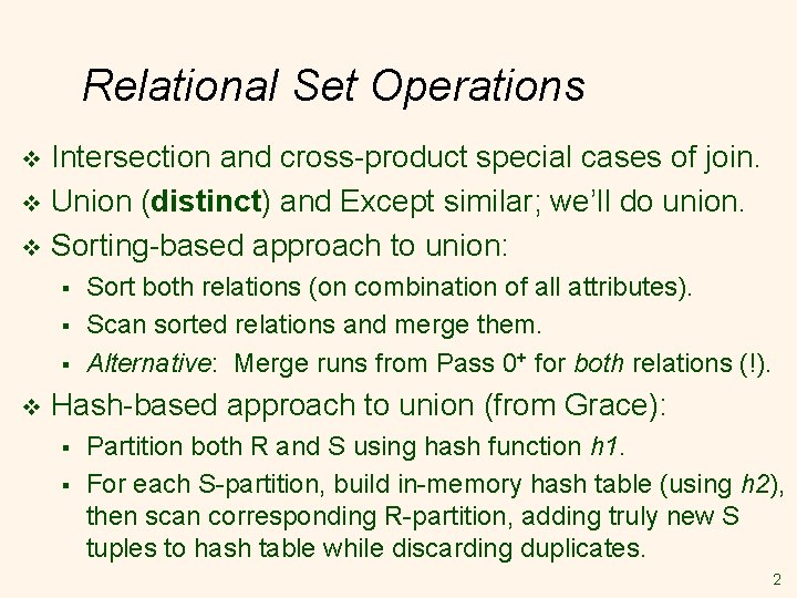
Relational Set Operations Intersection and cross-product special cases of join. v Union (distinct) and Except similar; we’ll do union. v Sorting-based approach to union: v § § § v Sort both relations (on combination of all attributes). Scan sorted relations and merge them. Alternative: Merge runs from Pass 0+ for both relations (!). Hash-based approach to union (from Grace): § § Partition both R and S using hash function h 1. For each S-partition, build in-memory hash table (using h 2), then scan corresponding R-partition, adding truly new S tuples to hash table while discarding duplicates. 2

Sets versus Bags UNION, INTERSECT, and DIFFERENCE (EXCEPT or MINUS) use the set semantics. v UNION ALL just combine two relations without considering any correlation. v 3

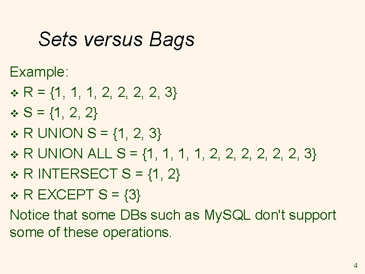
Sets versus Bags Example: v R = {1, 1, 1, 2, 2, 3} v S = {1, 2, 2} v R UNION S = {1, 2, 3} v R UNION ALL S = {1, 1, 2, 2, 2, 3} v R INTERSECT S = {1, 2} v R EXCEPT S = {3} Notice that some DBs such as My. SQL don't support some of these operations. 4

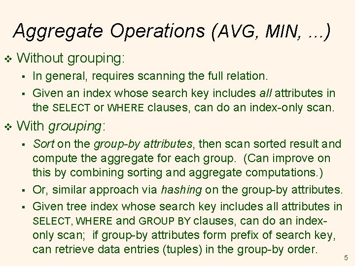
Aggregate Operations (AVG, MIN, . . . ) v Without grouping: § § v In general, requires scanning the full relation. Given an index whose search key includes all attributes in the SELECT or WHERE clauses, can do an index-only scan. With grouping: § § § Sort on the group-by attributes, then scan sorted result and compute the aggregate for each group. (Can improve on this by combining sorting and aggregate computations. ) Or, similar approach via hashing on the group-by attributes. Given tree index whose search key includes all attributes in SELECT, WHERE and GROUP BY clauses, can do an indexonly scan; if group-by attributes form prefix of search key, can retrieve data entries (tuples) in the group-by order. 5

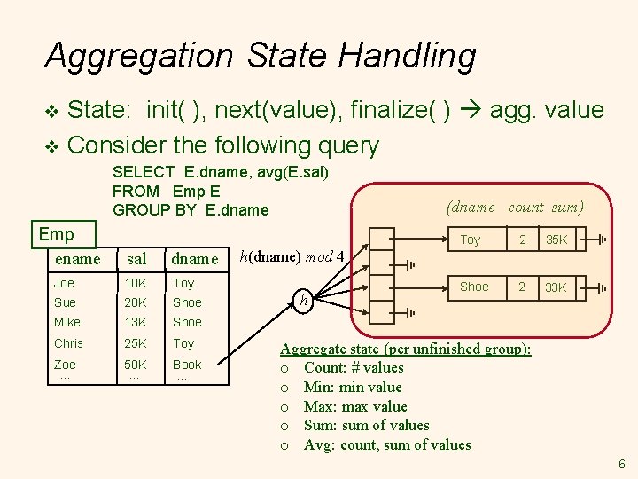
Aggregation State Handling State: init( ), next(value), finalize( ) agg. value v Consider the following query v SELECT E. dname, avg(E. sal) FROM Emp E GROUP BY E. dname Emp ename sal dname Joe 10 K Toy Sue 20 K Shoe Mike 13 K Shoe Chris 25 K Toy Zoe … 50 K … Book … (dname count sum) Toy 2 35 K Shoe 2 33 K h(dname) mod 4 h Aggregate state (per unfinished group): o Count: # values o Min: min value o Max: max value o Sum: sum of values o Avg: count, sum of values 6

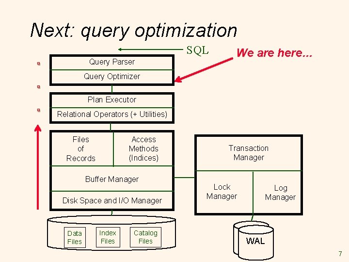
Next: query optimization SQL We are here…. . . Query Parser Query Optimizer Plan Executor Relational Operators (+ Utilities) Access Methods (Indices) Files of Records Buffer Manager Disk Space and I/O Manager Data Files Index Files Catalog Files Transaction Manager Lock Manager Log Manager WAL 7

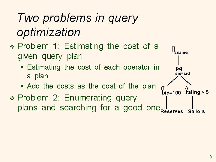
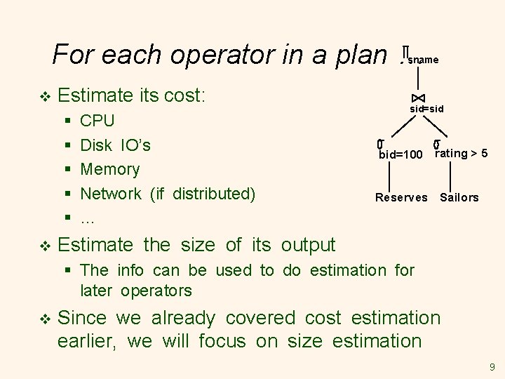
Two problems in query optimization v Problem 1: Estimating the cost of a given query plan § Estimating the cost of each operator in a plan § Add the costs as the cost of the plan v sname sid=sid bid=100 rating > 5 Problem 2: Enumerating query plans and searching for a good one. Reserves Sailors 8

For each operator in a plan … sname v Estimate its cost: § § § v CPU Disk IO’s Memory Network (if distributed) … sid=sid bid=100 rating > 5 Reserves Sailors Estimate the size of its output § The info can be used to do estimation for later operators v Since we already covered cost estimation earlier, we will focus on size estimation 9

Statistics in catalog v Optimizers use statistics in catalog to estimate the cardinalities of operators’ inputs and outputs § Simplifying assumptions: uniform distribution of attribute values, independence of attributes, etc. v For each relation R: § Cardinality of R (|R|), avg R-tuple width, and # of pages in R (||R||) – pick any 2 to know all 3 (given the page size) v For each (indexed) attribute of R: § § Number of distinct values |πA(R)| Range of values (i. e. , low and high values) Number of index leaf pages Number of index levels (if B+ tree) 10

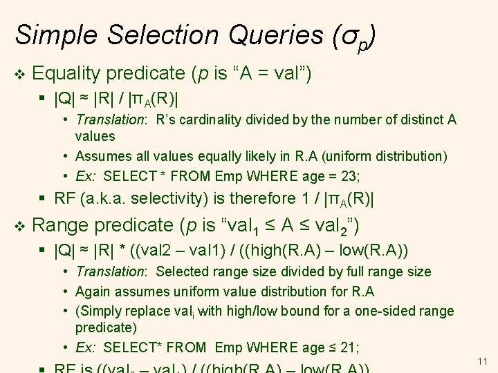
Simple Selection Queries (σp) v Equality predicate (p is “A = val”) § |Q| ≈ |R| / |πA(R)| • Translation: R’s cardinality divided by the number of distinct A values • Assumes all values equally likely in R. A (uniform distribution) • Ex: SELECT * FROM Emp WHERE age = 23; § RF (a. k. a. selectivity) is therefore 1 / |πA(R)| v Range predicate (p is “val 1 ≤ A ≤ val 2”) § |Q| ≈ |R| * ((val 2 – val 1) / ((high(R. A) – low(R. A)) • Translation: Selected range size divided by full range size • Again assumes uniform value distribution for R. A • (Simply replace vali with high/low bound for a one-sided range predicate) • Ex: SELECT* FROM Emp WHERE age ≤ 21; 11

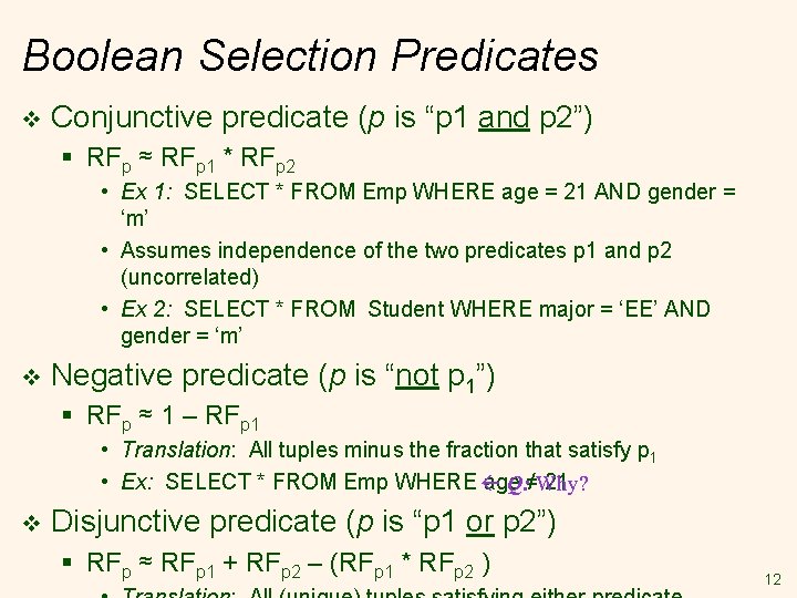
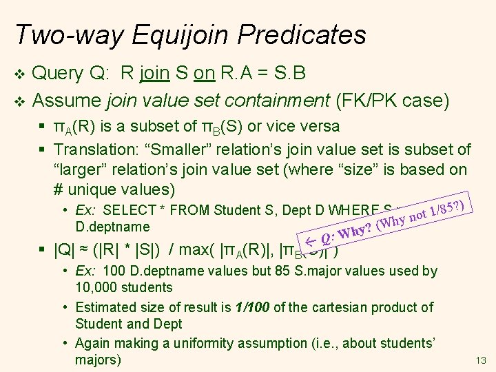
Boolean Selection Predicates v Conjunctive predicate (p is “p 1 and p 2”) § RFp ≈ RFp 1 * RFp 2 • Ex 1: SELECT * FROM Emp WHERE age = 21 AND gender = ‘m’ • Assumes independence of the two predicates p 1 and p 2 (uncorrelated) • Ex 2: SELECT * FROM Student WHERE major = ‘EE’ AND gender = ‘m’ v Negative predicate (p is “not p 1”) § RFp ≈ 1 – RFp 1 • Translation: All tuples minus the fraction that satisfy p 1 • Ex: SELECT * FROM Emp WHERE age 21 Q: ≠Why? v Disjunctive predicate (p is “p 1 or p 2”) § RFp ≈ RFp 1 + RFp 2 – (RFp 1 * RFp 2 ) 12

Two-way Equijoin Predicates Query Q: R join S on R. A = S. B v Assume join value set containment (FK/PK case) v § πA(R) is a subset of πB(S) or vice versa § Translation: “Smaller” relation’s join value set is subset of “larger” relation’s join value set (where “size” is based on # unique values) ? ) 5 8 / • Ex: SELECT * FROM Student S, Dept D WHERE S. major = 1 not y h D. deptname y? (W h W Q: § |Q| ≈ (|R| * |S|) / max( |πA(R)|, |πB(S)| ) • Ex: 100 D. deptname values but 85 S. major values used by 10, 000 students • Estimated size of result is 1/100 of the cartesian product of Student and Dept • Again making a uniformity assumption (i. e. , about students’ majors) 13

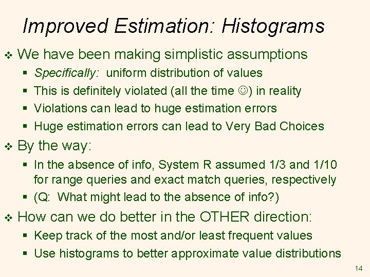
Improved Estimation: Histograms v We have been making simplistic assumptions § § v Specifically: uniform distribution of values This is definitely violated (all the time ) in reality Violations can lead to huge estimation errors Huge estimation errors can lead to Very Bad Choices By the way: § In the absence of info, System R assumed 1/3 and 1/10 for range queries and exact match queries, respectively § (Q: What might lead to the absence of info? ) v How can we do better in the OTHER direction: § Keep track of the most and/or least frequent values § Use histograms to better approximate value distributions 14

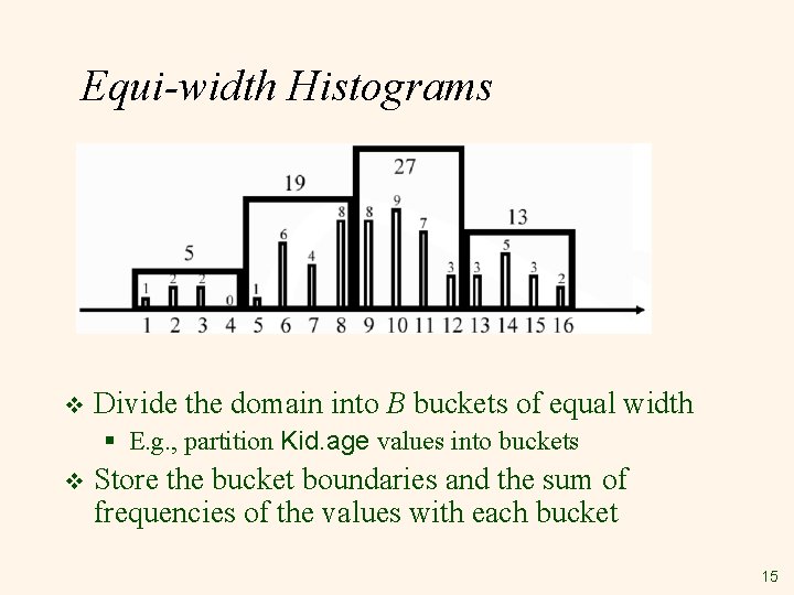
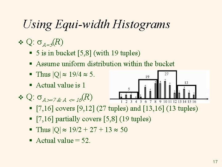
Equi-width Histograms v Divide the domain into B buckets of equal width § E. g. , partition Kid. age values into buckets v Store the bucket boundaries and the sum of frequencies of the values with each bucket 15

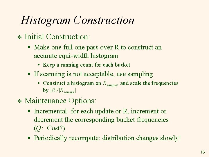
Histogram Construction v Initial Construction: § Make one full one pass over R to construct an accurate equi-width histogram • Keep a running count for each bucket § If scanning is not acceptable, use sampling • Construct a histogram on Rsample, and scale the frequencies by |R|/|Rsample| v Maintenance Options: § Incremental: for each update or R, increment or decrement the corresponding bucket frequencies (Q: Cost? ) § Periodically recompute: distribution changes slowly! 16

Using Equi-width Histograms v Q: s. A=5(R) § § v 5 is in bucket [5, 8] (with 19 tuples) Assume uniform distribution within the bucket Thus |Q| 19/4 5. Actual value is 1 Q: s. A>=7 & A <= 16(R) § § [7, 16] covers [9, 12] (27 tuples) and [13, 16] (13 tuples) [7, 16] partially covers [5, 8] (19 tuples) Thus |Q| 19/2 + 27 + 13 50 Actual value = 52. 17

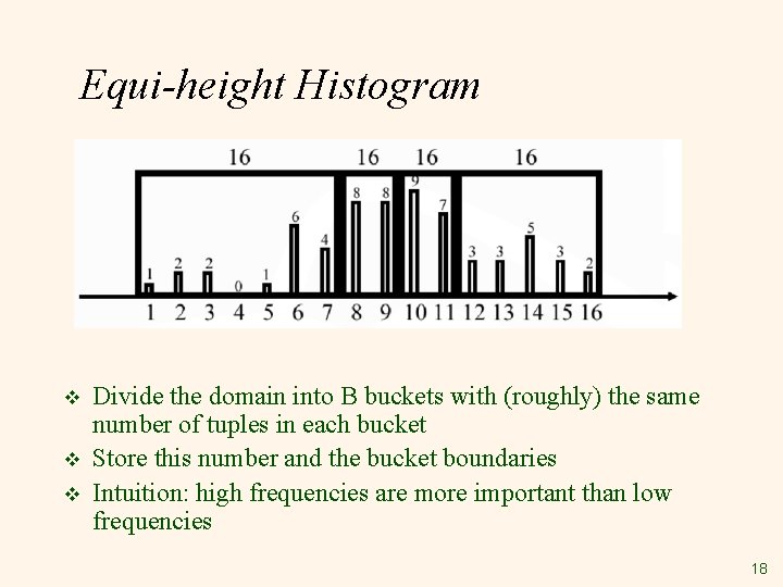
Equi-height Histogram v v v Divide the domain into B buckets with (roughly) the same number of tuples in each bucket Store this number and the bucket boundaries Intuition: high frequencies are more important than low frequencies 18

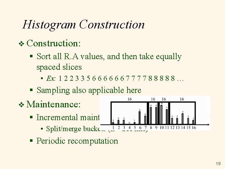
Histogram Construction v Construction: § Sort all R. A values, and then take equally spaced slices • Ex: 1 2 2 3 3 5 6 6 6 7 7 8 8 8 … § Sampling also applicable here v Maintenance: § Incremental maintenance • Split/merge buckets (B+ tree like) § Periodic recomputation 19

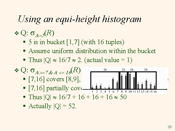
Using an equi-height histogram v Q: s. A=5(R) § 5 is in bucket [1, 7] (with 16 tuples) § Assume uniform distribution within the bucket § Thus |Q| 16/7 2. (actual value = 1) v Q: § § s. A>=7 & A <= 16(R) [7, 16] covers [8, 9], [10, 11], [12, 16] (all with tuples) [7, 16] partially covers [1, 7] (16 tuples) Thus |Q| 16/7 + 16 50 Actually |Q| = 52. 20

Can Combine Approaches v If values are badly skewed § Keep high/low frequency value information in addition to histograms § Could even apply the idea recursively: keep this sort of information for each bucket • “Divide” by converting values to some # ranges • “Conquer” by keeping some statistics for each range v Some “statistical glitches” to be aware of § Parameterized queries § Runtime situations 21