CS 162 Operating Systems and Systems Programming Lecture

CS 162 Operating Systems and Systems Programming Lecture 10 Language Support for Synchronization Scheduling February 26 th, 2019 Prof. John Kubiatowicz http: //cs 162. eecs. Berkeley. edu

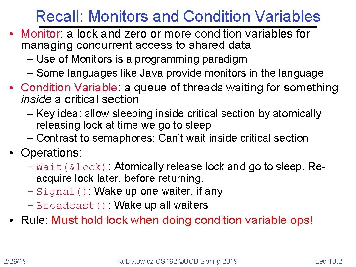
Recall: Monitors and Condition Variables • Monitor: a lock and zero or more condition variables for managing concurrent access to shared data – Use of Monitors is a programming paradigm – Some languages like Java provide monitors in the language • Condition Variable: a queue of threads waiting for something inside a critical section – Key idea: allow sleeping inside critical section by atomically releasing lock at time we go to sleep – Contrast to semaphores: Can’t wait inside critical section • Operations: – Wait(&lock): Atomically release lock and go to sleep. Reacquire lock later, before returning. – Signal(): Wake up one waiter, if any – Broadcast(): Wake up all waiters • Rule: Must hold lock when doing condition variable ops! 2/26/19 Kubiatowicz CS 162 ©UCB Spring 2019 Lec 10. 2

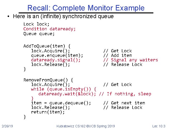
Recall: Complete Monitor Example • Here is an (infinite) synchronized queue Lock lock; Condition dataready; Queue queue; Add. To. Queue(item) { lock. Acquire(); queue. enqueue(item); dataready. signal(); lock. Release(); } // // Get Lock Add item Signal any waiters Release Lock Remove. From. Queue() { lock. Acquire(); // Get Lock while (queue. is. Empty()) { dataready. wait(&lock); // If nothing, sleep } item = queue. dequeue(); // Get next item lock. Release(); // Release Lock return(item); } 2/26/19 Kubiatowicz CS 162 ©UCB Spring 2019 Lec 10. 3

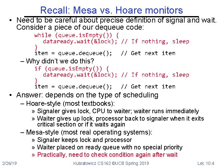
Recall: Mesa vs. Hoare monitors • Need to be careful about precise definition of signal and wait. Consider a piece of our dequeue code: while (queue. is. Empty()) { dataready. wait(&lock); // If nothing, sleep } item = queue. dequeue(); // Get next item – Why didn’t we do this? if (queue. is. Empty()) { dataready. wait(&lock); // If nothing, sleep } item = queue. dequeue(); // Get next item • Answer: depends on the type of scheduling – Hoare-style (most textbooks): » Signaler gives lock, CPU to waiter; waiter runs immediately » Waiter gives up lock, processor back to signaler when it exits critical section or if it waits again – Mesa-style (most real operating systems): » Signaler keeps lock and processor » Waiter placed on ready queue with no special priority » Practically, need to check condition again after wait 2/26/19 Kubiatowicz CS 162 ©UCB Spring 2019 Lec 10. 4

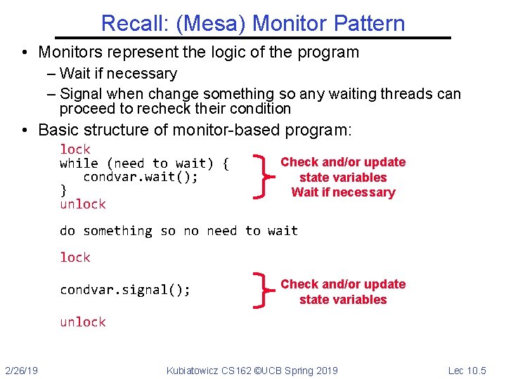
Recall: (Mesa) Monitor Pattern • Monitors represent the logic of the program – Wait if necessary – Signal when change something so any waiting threads can proceed to recheck their condition • Basic structure of monitor-based program: lock while (need to wait) { condvar. wait(); } unlock Check and/or update state variables Wait if necessary do something so no need to wait lock condvar. signal(); Check and/or update state variables unlock 2/26/19 Kubiatowicz CS 162 ©UCB Spring 2019 Lec 10. 5

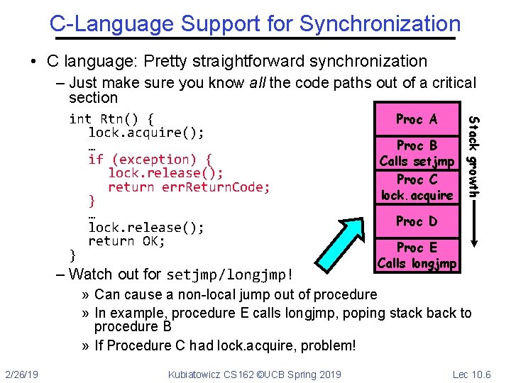
C-Language Support for Synchronization • C language: Pretty straightforward synchronization – Just make sure you know all the code paths out of a critical section – Watch out for setjmp/longjmp! Proc A Proc B Calls setjmp Proc C lock. acquire Stack growth int Rtn() { lock. acquire(); … if (exception) { lock. release(); return err. Return. Code; } … lock. release(); return OK; } Proc D Proc E Calls longjmp » Can cause a non-local jump out of procedure » In example, procedure E calls longjmp, poping stack back to procedure B » If Procedure C had lock. acquire, problem! 2/26/19 Kubiatowicz CS 162 ©UCB Spring 2019 Lec 10. 6

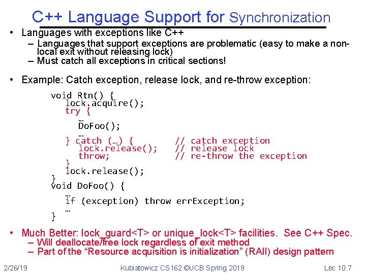
C++ Language Support for Synchronization • Languages with exceptions like C++ – Languages that support exceptions are problematic (easy to make a nonlocal exit without releasing lock) – Must catch all exceptions in critical sections! • Example: Catch exception, release lock, and re-throw exception: void Rtn() { lock. acquire(); try { … Do. Foo(); … } catch (…) { lock. release(); throw; } lock. release(); } void Do. Foo() { … if (exception) throw … } // catch exception // release lock // re-throw the exception err. Exception; • Much Better: lock_guard<T> or unique_lock<T> facilities. See C++ Spec. – Will deallocate/free lock regardless of exit method – Part of the “Resource acquisition is initialization” (RAII) design pattern 2/26/19 Kubiatowicz CS 162 ©UCB Spring 2019 Lec 10. 7

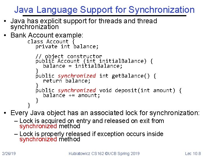
Java Language Support for Synchronization • Java has explicit support for threads and thread synchronization • Bank Account example: class Account { private int balance; } // object constructor public Account (int initial. Balance) { balance = initial. Balance; } public synchronized int get. Balance() { return balance; } public synchronized void deposit(int amount) { balance += amount; } • Every Java object has an associated lock for synchronization: – Lock is acquired on entry and released on exit from synchronized method – Lock is properly released if exception occurs inside synchronized method 2/26/19 Kubiatowicz CS 162 ©UCB Spring 2019 Lec 10. 8

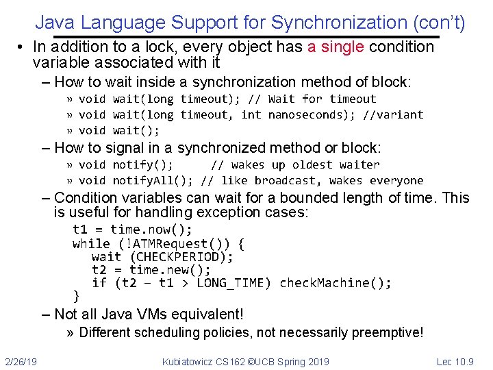
Java Language Support for Synchronization (con’t) • In addition to a lock, every object has a single condition variable associated with it – How to wait inside a synchronization method of block: » void wait(long timeout); // Wait for timeout » void wait(long timeout, int nanoseconds); //variant » void wait(); – How to signal in a synchronized method or block: » void notify(); // wakes up oldest waiter » void notify. All(); // like broadcast, wakes everyone – Condition variables can wait for a bounded length of time. This is useful for handling exception cases: t 1 = time. now(); while (!ATMRequest()) { wait (CHECKPERIOD); t 2 = time. new(); if (t 2 – t 1 > LONG_TIME) check. Machine(); } – Not all Java VMs equivalent! » Different scheduling policies, not necessarily preemptive! 2/26/19 Kubiatowicz CS 162 ©UCB Spring 2019 Lec 10. 9

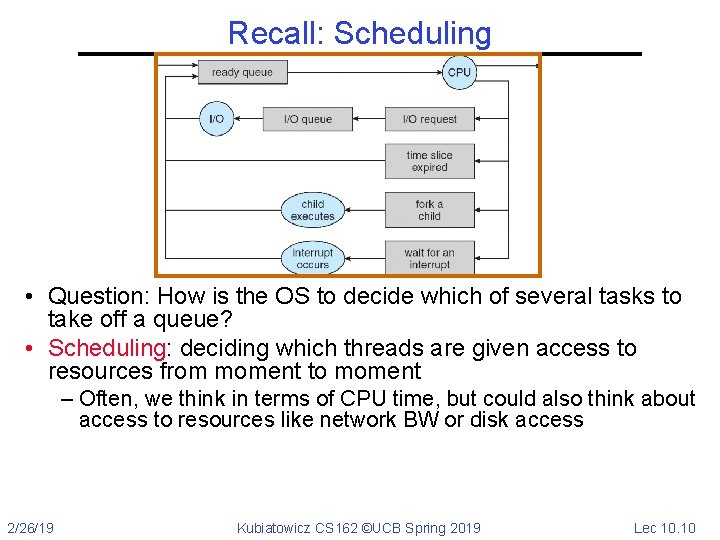
Recall: Scheduling • Question: How is the OS to decide which of several tasks to take off a queue? • Scheduling: deciding which threads are given access to resources from moment to moment – Often, we think in terms of CPU time, but could also think about access to resources like network BW or disk access 2/26/19 Kubiatowicz CS 162 ©UCB Spring 2019 Lec 10. 10

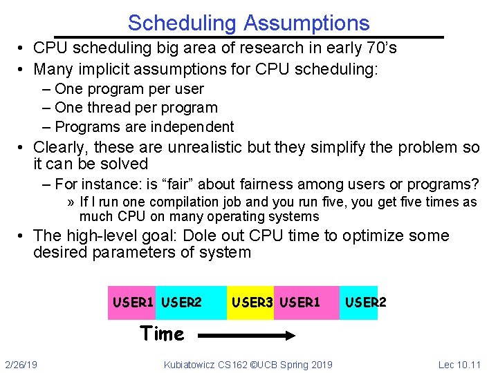
Scheduling Assumptions • CPU scheduling big area of research in early 70’s • Many implicit assumptions for CPU scheduling: – One program per user – One thread per program – Programs are independent • Clearly, these are unrealistic but they simplify the problem so it can be solved – For instance: is “fair” about fairness among users or programs? » If I run one compilation job and you run five, you get five times as much CPU on many operating systems • The high-level goal: Dole out CPU time to optimize some desired parameters of system USER 1 USER 2 USER 3 USER 1 USER 2 Time 2/26/19 Kubiatowicz CS 162 ©UCB Spring 2019 Lec 10. 11

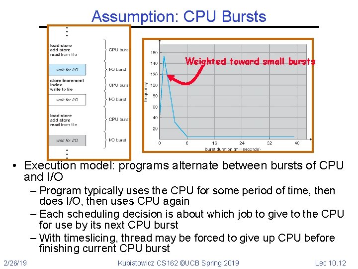
Assumption: CPU Bursts Weighted toward small bursts • Execution model: programs alternate between bursts of CPU and I/O – Program typically uses the CPU for some period of time, then does I/O, then uses CPU again – Each scheduling decision is about which job to give to the CPU for use by its next CPU burst – With timeslicing, thread may be forced to give up CPU before finishing current CPU burst 2/26/19 Kubiatowicz CS 162 ©UCB Spring 2019 Lec 10. 12

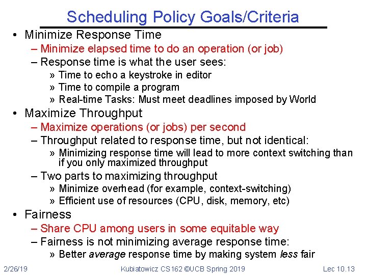
Scheduling Policy Goals/Criteria • Minimize Response Time – Minimize elapsed time to do an operation (or job) – Response time is what the user sees: » Time to echo a keystroke in editor » Time to compile a program » Real-time Tasks: Must meet deadlines imposed by World • Maximize Throughput – Maximize operations (or jobs) per second – Throughput related to response time, but not identical: » Minimizing response time will lead to more context switching than if you only maximized throughput – Two parts to maximizing throughput » Minimize overhead (for example, context-switching) » Efficient use of resources (CPU, disk, memory, etc) • Fairness – Share CPU among users in some equitable way – Fairness is not minimizing average response time: » Better average response time by making system less fair 2/26/19 Kubiatowicz CS 162 ©UCB Spring 2019 Lec 10. 13

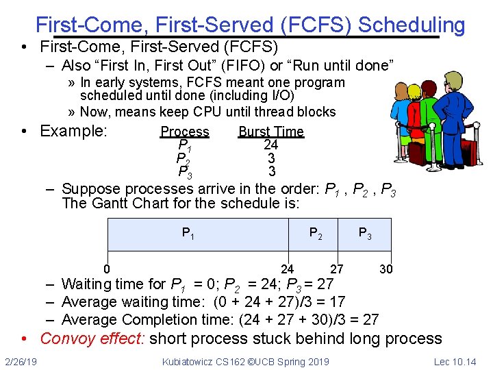
First-Come, First-Served (FCFS) Scheduling • First-Come, First-Served (FCFS) – Also “First In, First Out” (FIFO) or “Run until done” » In early systems, FCFS meant one program scheduled until done (including I/O) » Now, means keep CPU until thread blocks • Example: Process Burst Time P 1 24 P 2 3 P 3 3 – Suppose processes arrive in the order: P 1 , P 2 , P 3 The Gantt Chart for the schedule is: P 1 0 P 2 24 P 3 27 30 – Waiting time for P 1 = 0; P 2 = 24; P 3 = 27 – Average waiting time: (0 + 24 + 27)/3 = 17 – Average Completion time: (24 + 27 + 30)/3 = 27 • Convoy effect: short process stuck behind long process 2/26/19 Kubiatowicz CS 162 ©UCB Spring 2019 Lec 10. 14

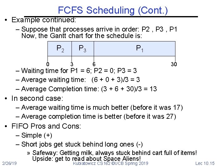
FCFS Scheduling (Cont. ) • Example continued: – Suppose that processes arrive in order: P 2 , P 3 , P 1 Now, the Gantt chart for the schedule is: P 2 0 P 3 3 P 1 6 – Waiting time for P 1 = 6; P 2 = 0; P 3 = 3 – Average waiting time: (6 + 0 + 3)/3 = 3 – Average Completion time: (3 + 6 + 30)/3 = 13 30 • In second case: – Average waiting time is much better (before it was 17) – Average completion time is better (before it was 27) • FIFO Pros and Cons: – Simple (+) – Short jobs get stuck behind long ones (-) 2/26/19 » Safeway: Getting milk, always stuck behind cart full of items! Upside: get to read about Space Aliens! Kubiatowicz CS 162 ©UCB Spring 2019 Lec 10. 15

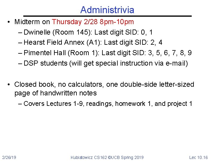
Administrivia • Midterm on Thursday 2/28 8 pm-10 pm – Dwinelle (Room 145): Last digit SID: 0, 1 – Hearst Field Annex (A 1): Last digit SID: 2, 4 – Pimentel Hall (Room 1): Last digit SID: 3, 5, 6, 7, 8, 9 – DSP students (will get special instruction via e-mail) • Closed book, no calculators, one double-side letter-sized page of handwritten notes – Covers Lectures 1 -9, readings, homework 1, and project 1 2/26/19 Kubiatowicz CS 162 ©UCB Spring 2019 Lec 10. 16

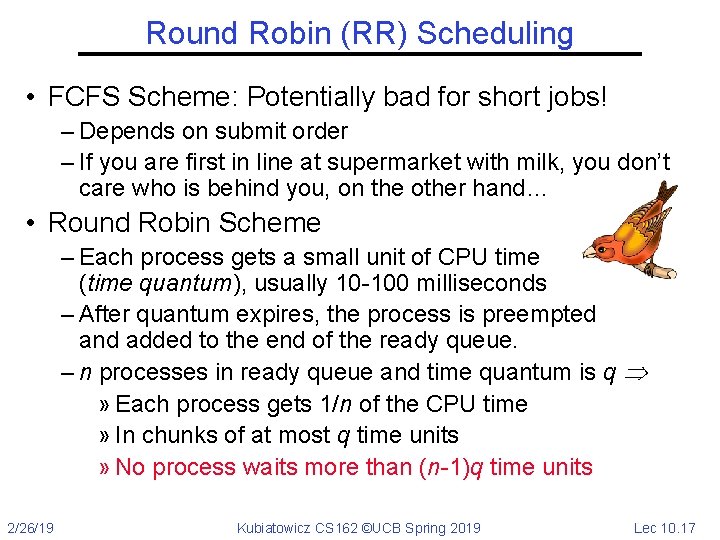
Round Robin (RR) Scheduling • FCFS Scheme: Potentially bad for short jobs! – Depends on submit order – If you are first in line at supermarket with milk, you don’t care who is behind you, on the other hand… • Round Robin Scheme – Each process gets a small unit of CPU time (time quantum), usually 10 -100 milliseconds – After quantum expires, the process is preempted and added to the end of the ready queue. – n processes in ready queue and time quantum is q » Each process gets 1/n of the CPU time » In chunks of at most q time units » No process waits more than (n-1)q time units 2/26/19 Kubiatowicz CS 162 ©UCB Spring 2019 Lec 10. 17

RR Scheduling (Cont. ) • Performance – q large FCFS – q small Interleaved (really small hyperthreading? ) – q must be large with respect to context switch, otherwise overhead is too high (all overhead) 2/26/19 Kubiatowicz CS 162 ©UCB Spring 2019 Lec 10. 18

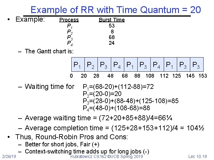
Example of RR with Time Quantum = 20 • Example: Process P 1 P 2 P 3 P 4 Burst Time 53 8 68 24 – The Gantt chart is: P 1 P 2 P 3 P 4 P 1 P 3 0 20 28 48 68 88 108 112 125 145 153 – Waiting time for P 1=(68 -20)+(112 -88)=72 P 2=(20 -0)=20 P 3=(28 -0)+(88 -48)+(125 -108)=85 P 4=(48 -0)+(108 -68)=88 – Average waiting time = (72+20+85+88)/4=66¼ – Average completion time = (125+28+153+112)/4 = 104½ • Thus, Round-Robin Pros and Cons: 2/26/19 – Better for short jobs, Fair (+) – Context-switching time adds up for long jobs (-) Kubiatowicz CS 162 ©UCB Spring 2019 Lec 10. 19

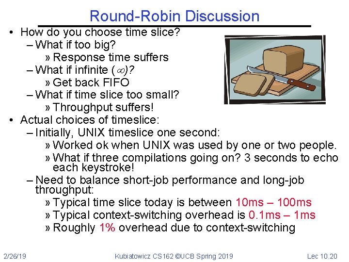
Round-Robin Discussion • How do you choose time slice? – What if too big? » Response time suffers – What if infinite ( )? » Get back FIFO – What if time slice too small? » Throughput suffers! • Actual choices of timeslice: – Initially, UNIX timeslice one second: » Worked ok when UNIX was used by one or two people. » What if three compilations going on? 3 seconds to echo each keystroke! – Need to balance short-job performance and long-job throughput: » Typical time slice today is between 10 ms – 100 ms » Typical context-switching overhead is 0. 1 ms – 1 ms » Roughly 1% overhead due to context-switching 2/26/19 Kubiatowicz CS 162 ©UCB Spring 2019 Lec 10. 20

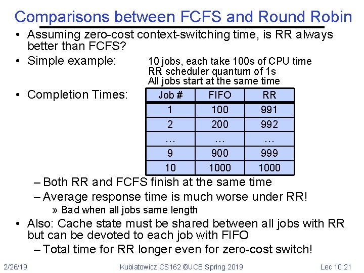
Comparisons between FCFS and Round Robin • Assuming zero-cost context-switching time, is RR always better than FCFS? • Simple example: 10 jobs, each take 100 s of CPU time • Completion Times: RR scheduler quantum of 1 s All jobs start at the same time Job # FIFO RR 1 100 991 2 200 992 … … … 9 900 999 10 1000 – Both RR and FCFS finish at the same time – Average response time is much worse under RR! » Bad when all jobs same length • Also: Cache state must be shared between all jobs with RR but can be devoted to each job with FIFO – Total time for RR longer even for zero-cost switch! 2/26/19 Kubiatowicz CS 162 ©UCB Spring 2019 Lec 10. 21

Earlier Example with Different Time Quantum P 2 P 4 Best FCFS: [8] [24] 0 32 8 Quantum Best FCFS Q = 1 Q = 5 Wait Q = 8 Time Q = 10 Q = 20 Worst FCFS Best FCFS Q = 1 Q = 5 Completion Q = 8 Time Q = 10 Q = 20 Worst FCFS 2/26/19 P 1 [53] P 3 [68] 85 153 P 1 P 2 P 3 P 4 Average 32 84 82 80 82 72 68 85 137 135 133 135 121 0 22 20 8 10 20 145 8 30 28 16 18 28 153 85 85 85 0 153 153 153 68 8 57 58 56 68 88 121 32 81 82 80 92 112 145 31¼ 62 61¼ 57¼ 61¼ 66¼ 83½ 69½ 100½ 99½ 95½ 99½ 104½ 121¾ Kubiatowicz CS 162 ©UCB Spring 2019 Lec 10. 22

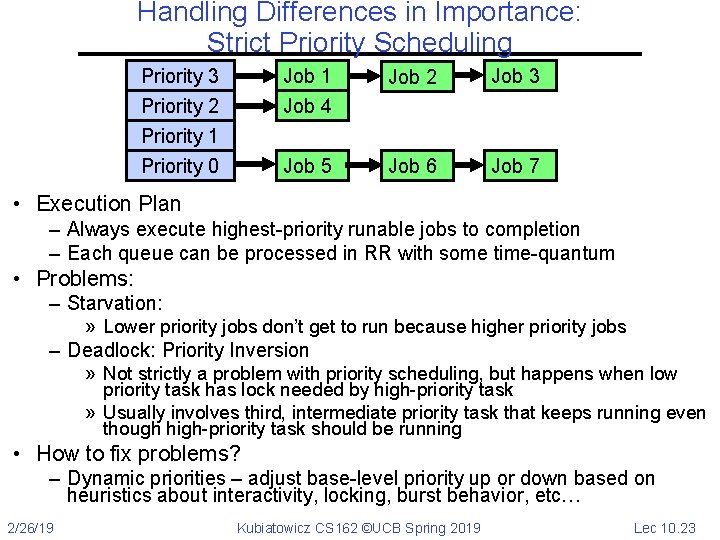
Handling Differences in Importance: Strict Priority Scheduling Priority 3 Priority 2 Priority 1 Job 4 Job 2 Job 3 Priority 0 Job 5 Job 6 Job 7 • Execution Plan – Always execute highest-priority runable jobs to completion – Each queue can be processed in RR with some time-quantum • Problems: – Starvation: » Lower priority jobs don’t get to run because higher priority jobs – Deadlock: Priority Inversion » Not strictly a problem with priority scheduling, but happens when low priority task has lock needed by high-priority task » Usually involves third, intermediate priority task that keeps running even though high-priority task should be running • How to fix problems? – Dynamic priorities – adjust base-level priority up or down based on heuristics about interactivity, locking, burst behavior, etc… 2/26/19 Kubiatowicz CS 162 ©UCB Spring 2019 Lec 10. 23

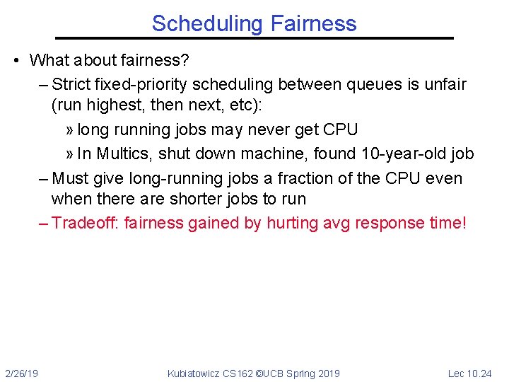
Scheduling Fairness • What about fairness? – Strict fixed-priority scheduling between queues is unfair (run highest, then next, etc): » long running jobs may never get CPU » In Multics, shut down machine, found 10 -year-old job – Must give long-running jobs a fraction of the CPU even when there are shorter jobs to run – Tradeoff: fairness gained by hurting avg response time! 2/26/19 Kubiatowicz CS 162 ©UCB Spring 2019 Lec 10. 24

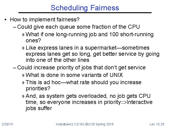
Scheduling Fairness • How to implement fairness? – Could give each queue some fraction of the CPU » What if one long-running job and 100 short-running ones? » Like express lanes in a supermarket—sometimes express lanes get so long, get better service by going into one of the other lines – Could increase priority of jobs that don’t get service » What is done in some variants of UNIX » This is ad hoc—what rate should you increase priorities? » And, as system gets overloaded, no job gets CPU time, so everyone increases in priority Interactive jobs suffer 2/26/19 Kubiatowicz CS 162 ©UCB Spring 2019 Lec 10. 25

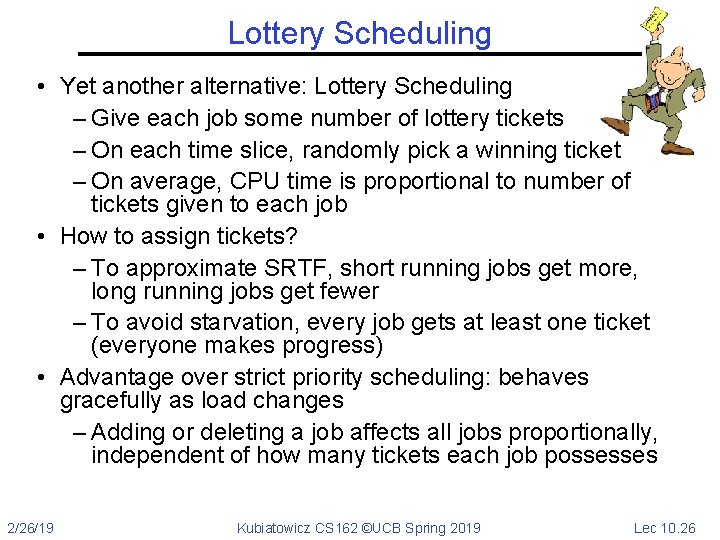
Lottery Scheduling • Yet another alternative: Lottery Scheduling – Give each job some number of lottery tickets – On each time slice, randomly pick a winning ticket – On average, CPU time is proportional to number of tickets given to each job • How to assign tickets? – To approximate SRTF, short running jobs get more, long running jobs get fewer – To avoid starvation, every job gets at least one ticket (everyone makes progress) • Advantage over strict priority scheduling: behaves gracefully as load changes – Adding or deleting a job affects all jobs proportionally, independent of how many tickets each job possesses 2/26/19 Kubiatowicz CS 162 ©UCB Spring 2019 Lec 10. 26

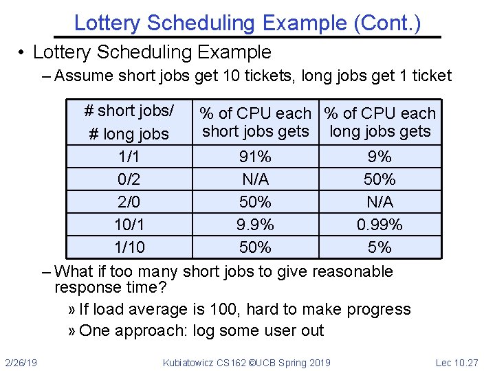
Lottery Scheduling Example (Cont. ) • Lottery Scheduling Example – Assume short jobs get 10 tickets, long jobs get 1 ticket # short jobs/ % of CPU each short jobs gets long jobs gets # long jobs 1/1 91% 9% 0/2 N/A 50% 2/0 50% N/A 10/1 9. 9% 0. 99% 1/10 50% 5% – What if too many short jobs to give reasonable response time? » If load average is 100, hard to make progress » One approach: log some user out 2/26/19 Kubiatowicz CS 162 ©UCB Spring 2019 Lec 10. 27

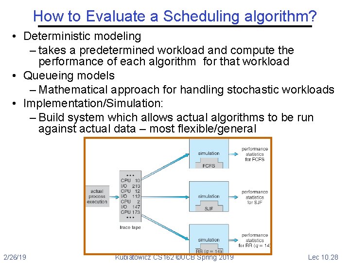
How to Evaluate a Scheduling algorithm? • Deterministic modeling – takes a predetermined workload and compute the performance of each algorithm for that workload • Queueing models – Mathematical approach for handling stochastic workloads • Implementation/Simulation: – Build system which allows actual algorithms to be run against actual data – most flexible/general 2/26/19 Kubiatowicz CS 162 ©UCB Spring 2019 Lec 10. 28

How to Handle Simultaneous Mix of Diff Types of Apps? • Consider mix of interactive and high throughput apps: – How to best schedule them? – How to recognize one from the other? » Do you trust app to say that it is “interactive”? – Should you schedule the set of apps identically on servers, workstations, pads, and cellphones? • For instance, is Burst Time (observed) useful to decide which application gets CPU time? – Short Bursts Interactivity High Priority? • Assumptions encoded into many schedulers: – Apps that sleep a lot and have short bursts must be interactive apps – they should get high priority – Apps that compute a lot should get low(er? ) priority, since they won’t notice intermittent bursts from interactive apps • Hard to characterize apps: 2/26/19 – What about apps that sleep for a long time, but then compute for a long time? – Or, what about apps that must run under all circumstances (say periodically) Kubiatowicz CS 162 ©UCB Spring 2019 Lec 10. 29

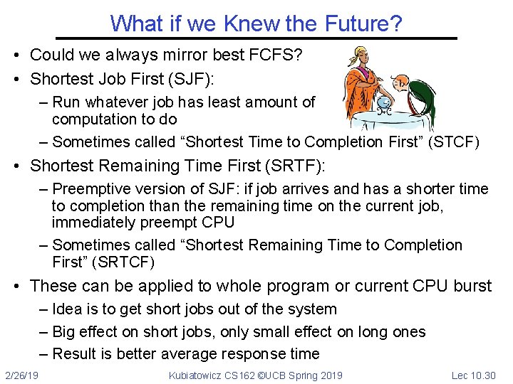
What if we Knew the Future? • Could we always mirror best FCFS? • Shortest Job First (SJF): – Run whatever job has least amount of computation to do – Sometimes called “Shortest Time to Completion First” (STCF) • Shortest Remaining Time First (SRTF): – Preemptive version of SJF: if job arrives and has a shorter time to completion than the remaining time on the current job, immediately preempt CPU – Sometimes called “Shortest Remaining Time to Completion First” (SRTCF) • These can be applied to whole program or current CPU burst – Idea is to get short jobs out of the system – Big effect on short jobs, only small effect on long ones – Result is better average response time 2/26/19 Kubiatowicz CS 162 ©UCB Spring 2019 Lec 10. 30

Discussion • SJF/SRTF are the best you can do at minimizing average response time – Provably optimal (SJF among non-preemptive, SRTF among preemptive) – Since SRTF is always at least as good as SJF, focus on SRTF • Comparison of SRTF with FCFS – What if all jobs the same length? » SRTF becomes the same as FCFS (i. e. FCFS is best can do if all jobs the same length) – What if jobs have varying length? » SRTF: short jobs not stuck behind long ones 2/26/19 Kubiatowicz CS 162 ©UCB Spring 2019 Lec 10. 31

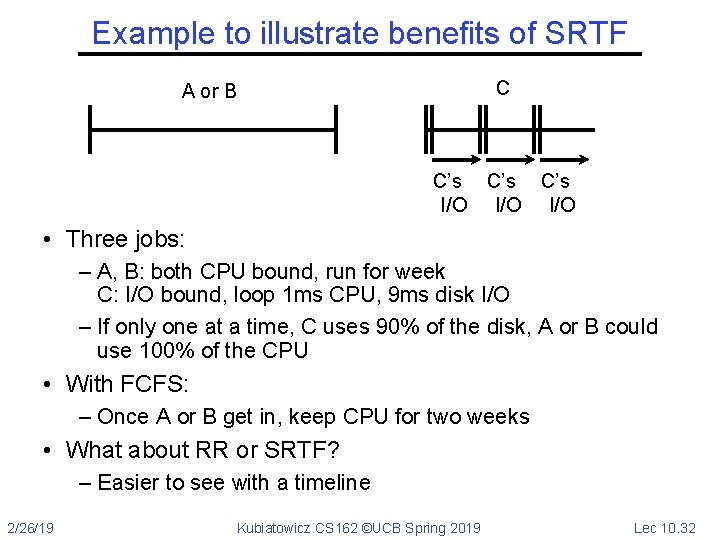
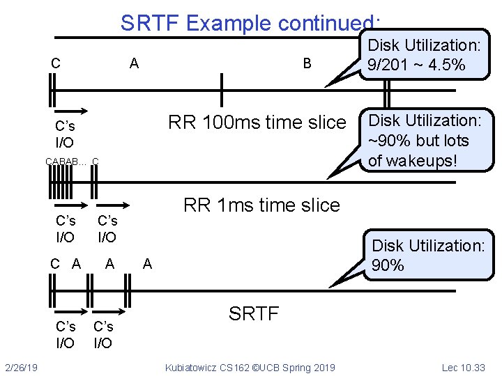
Example to illustrate benefits of SRTF C A or B C’s C’s I/O I/O • Three jobs: – A, B: both CPU bound, run for week C: I/O bound, loop 1 ms CPU, 9 ms disk I/O – If only one at a time, C uses 90% of the disk, A or B could use 100% of the CPU • With FCFS: – Once A or B get in, keep CPU for two weeks • What about RR or SRTF? – Easier to see with a timeline 2/26/19 Kubiatowicz CS 162 ©UCB Spring 2019 Lec 10. 32

SRTF Example continued: C A B RR 100 ms time slice C’s I/O CABAB… C C’s I/O C A A C’s I/O 2/26/19 Disk Utilization: C 9/201 ~ 4. 5% Disk Utilization: C’s ~90% but lots I/O of wakeups! RR 1 ms time slice Disk Utilization: 90% A SRTF Kubiatowicz CS 162 ©UCB Spring 2019 Lec 10. 33

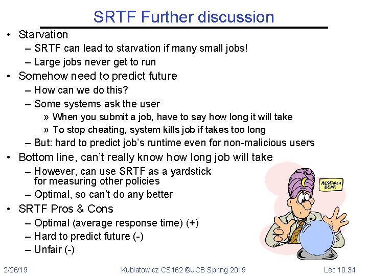
SRTF Further discussion • Starvation – SRTF can lead to starvation if many small jobs! – Large jobs never get to run • Somehow need to predict future – How can we do this? – Some systems ask the user » When you submit a job, have to say how long it will take » To stop cheating, system kills job if takes too long – But: hard to predict job’s runtime even for non-malicious users • Bottom line, can’t really know how long job will take – However, can use SRTF as a yardstick for measuring other policies – Optimal, so can’t do any better • SRTF Pros & Cons – Optimal (average response time) (+) – Hard to predict future (-) – Unfair (-) 2/26/19 Kubiatowicz CS 162 ©UCB Spring 2019 Lec 10. 34

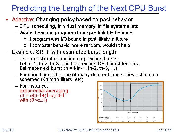
Predicting the Length of the Next CPU Burst • Adaptive: Changing policy based on past behavior – CPU scheduling, in virtual memory, in file systems, etc – Works because programs have predictable behavior » If program was I/O bound in past, likely in future » If computer behavior were random, wouldn’t help • Example: SRTF with estimated burst length – Use an estimator function on previous bursts: Let tn-1, tn-2, tn-3, etc. be previous CPU burst lengths. Estimate next burst n = f(tn-1, tn-2, tn-3, …) – Function f could be one of many different time series estimation schemes (Kalman filters, etc) – For instance, exponential averaging n = tn-1+(1 - ) n-1 with (0< 1) 2/26/19 Kubiatowicz CS 162 ©UCB Spring 2019 Lec 10. 35

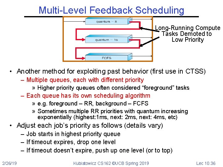
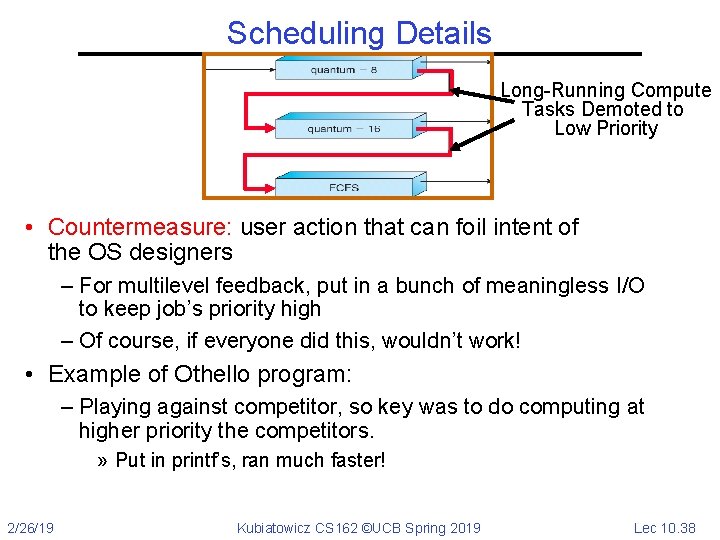
Multi-Level Feedback Scheduling Long-Running Compute Tasks Demoted to Low Priority • Another method for exploiting past behavior (first use in CTSS) – Multiple queues, each with different priority » Higher priority queues often considered “foreground” tasks – Each queue has its own scheduling algorithm » e. g. foreground – RR, background – FCFS » Sometimes multiple RR priorities with quantum increasing exponentially (highest: 1 ms, next: 2 ms, next: 4 ms, etc) • Adjust each job’s priority as follows (details vary) – Job starts in highest priority queue – If timeout expires, drop one level – If timeout doesn’t expire, push up one level (or to top) 2/26/19 Kubiatowicz CS 162 ©UCB Spring 2019 Lec 10. 36

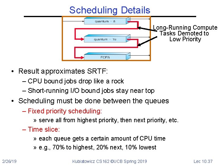
Scheduling Details Long-Running Compute Tasks Demoted to Low Priority • Result approximates SRTF: – CPU bound jobs drop like a rock – Short-running I/O bound jobs stay near top • Scheduling must be done between the queues – Fixed priority scheduling: » serve all from highest priority, then next priority, etc. – Time slice: » each queue gets a certain amount of CPU time » e. g. , 70% to highest, 20% next, 10% lowest 2/26/19 Kubiatowicz CS 162 ©UCB Spring 2019 Lec 10. 37

Scheduling Details Long-Running Compute Tasks Demoted to Low Priority • Countermeasure: user action that can foil intent of the OS designers – For multilevel feedback, put in a bunch of meaningless I/O to keep job’s priority high – Of course, if everyone did this, wouldn’t work! • Example of Othello program: – Playing against competitor, so key was to do computing at higher priority the competitors. » Put in printf’s, ran much faster! 2/26/19 Kubiatowicz CS 162 ©UCB Spring 2019 Lec 10. 38

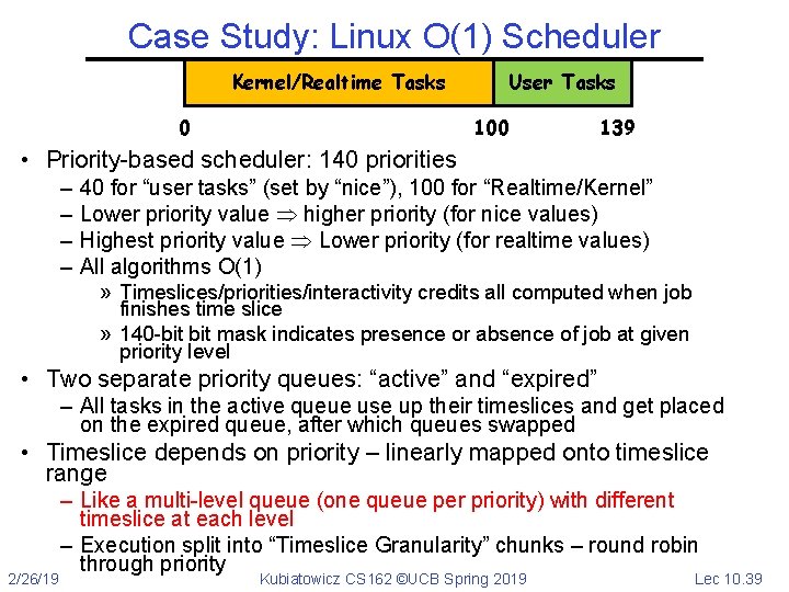
Case Study: Linux O(1) Scheduler Kernel/Realtime Tasks 0 User Tasks 100 139 • Priority-based scheduler: 140 priorities – – 40 for “user tasks” (set by “nice”), 100 for “Realtime/Kernel” Lower priority value higher priority (for nice values) Highest priority value Lower priority (for realtime values) All algorithms O(1) » Timeslices/priorities/interactivity credits all computed when job finishes time slice » 140 -bit mask indicates presence or absence of job at given priority level • Two separate priority queues: “active” and “expired” – All tasks in the active queue use up their timeslices and get placed on the expired queue, after which queues swapped • Timeslice depends on priority – linearly mapped onto timeslice range 2/26/19 – Like a multi-level queue (one queue per priority) with different timeslice at each level – Execution split into “Timeslice Granularity” chunks – round robin through priority Kubiatowicz CS 162 ©UCB Spring 2019 Lec 10. 39

O(1) Scheduler Continued • Heuristics – User-task priority adjusted ± 5 based on heuristics » p->sleep_avg = sleep_time – run_time » Higher sleep_avg more I/O bound the task, more reward (and vice versa) – Interactive Credit » Earned when a task sleeps for a “long” time » Spend when a task runs for a “long” time » IC is used to provide hysteresis to avoid changing interactivity for temporary changes in behavior – However, “interactive tasks” get special dispensation » To try to maintain interactivity » Placed back into active queue, unless some other task has been starved for too long… • Real-Time Tasks – Always preempt non-RT tasks – No dynamic adjustment of priorities – Scheduling schemes: » SCHED_FIFO: preempts other tasks, no timeslice limit » SCHED_RR: preempts normal tasks, RR scheduling amongst tasks of same priority 2/26/19 Kubiatowicz CS 162 ©UCB Spring 2019 Lec 10. 40

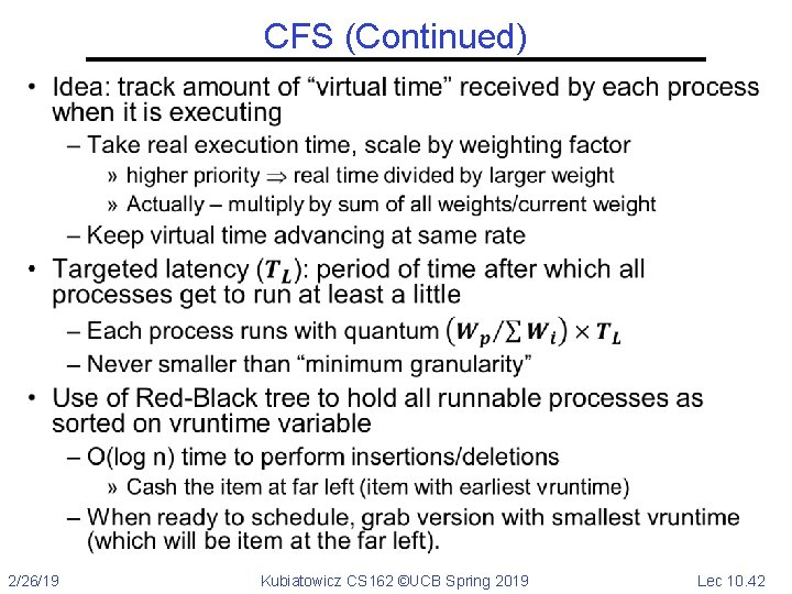
Linux Completely Fair Scheduler (CFS) • First appeared in 2. 6. 23, modified in 2. 6. 24 • “CFS doesn't track sleeping time and doesn't use heuristics to identify interactive tasks—it just makes sure every process gets a fair share of CPU within a set amount of time given the number of runnable processes on the CPU. ” • Inspired by Networking “Fair Queueing” – Each process given their fair share of resources – Models an “ideal multitasking processor” in which N processes execute simultaneously as if they truly got 1/N of the processor » Tries to give each process an equal fraction of the processor – Priorities reflected by weights such that increasing a task’s priority by 1 always gives the same fractional increase in CPU time – regardless of current priority 2/26/19 Kubiatowicz CS 162 ©UCB Spring 2019 Lec 10. 41

CFS (Continued) • 2/26/19 Kubiatowicz CS 162 ©UCB Spring 2019 Lec 10. 42

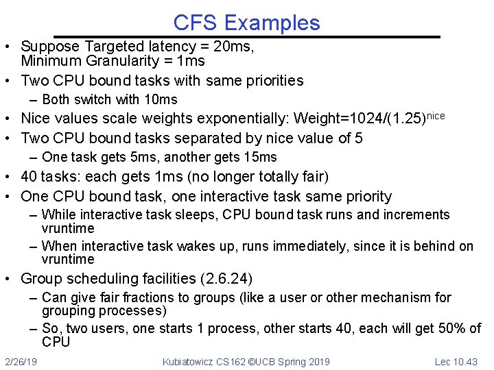
CFS Examples • Suppose Targeted latency = 20 ms, Minimum Granularity = 1 ms • Two CPU bound tasks with same priorities – Both switch with 10 ms • Nice values scale weights exponentially: Weight=1024/(1. 25)nice • Two CPU bound tasks separated by nice value of 5 – One task gets 5 ms, another gets 15 ms • 40 tasks: each gets 1 ms (no longer totally fair) • One CPU bound task, one interactive task same priority – While interactive task sleeps, CPU bound task runs and increments vruntime – When interactive task wakes up, runs immediately, since it is behind on vruntime • Group scheduling facilities (2. 6. 24) – Can give fair fractions to groups (like a user or other mechanism for grouping processes) – So, two users, one starts 1 process, other starts 40, each will get 50% of CPU 2/26/19 Kubiatowicz CS 162 ©UCB Spring 2019 Lec 10. 43

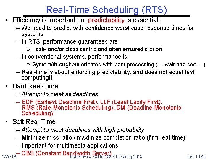
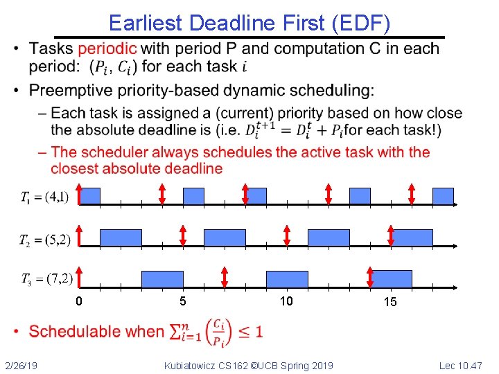
Real-Time Scheduling (RTS) • Efficiency is important but predictability is essential: – We need to predict with confidence worst case response times for systems – In RTS, performance guarantees are: » Task- and/or class centric and often ensured a priori – In conventional systems, performance is: » System/throughput oriented with post-processing (… wait and see …) – Real-time is about enforcing predictability, and does not equal fast computing!!! • Hard Real-Time – Attempt to meet all deadlines – EDF (Earliest Deadline First), LLF (Least Laxity First), RMS (Rate-Monotonic Scheduling), DM (Deadline Monotonic Scheduling) • Soft Real-Time – – 2/26/19 Attempt to meet deadlines with high probability Minimize miss ratio / maximize completion ratio (firm real-time) Important for multimedia applications CBS (Constant Bandwidth Server) Kubiatowicz CS 162 ©UCB Spring 2019 Lec 10. 44

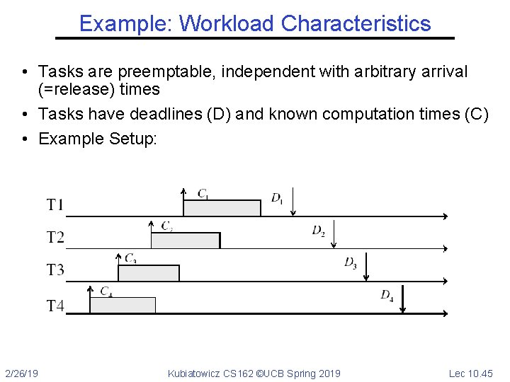
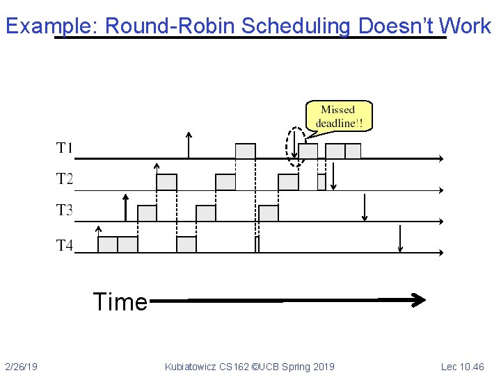
Example: Workload Characteristics • Tasks are preemptable, independent with arbitrary arrival (=release) times • Tasks have deadlines (D) and known computation times (C) • Example Setup: 2/26/19 Kubiatowicz CS 162 ©UCB Spring 2019 Lec 10. 45

Example: Round-Robin Scheduling Doesn’t Work Time 2/26/19 Kubiatowicz CS 162 ©UCB Spring 2019 Lec 10. 46

Earliest Deadline First (EDF) • 0 2/26/19 5 10 Kubiatowicz CS 162 ©UCB Spring 2019 15 Lec 10. 47

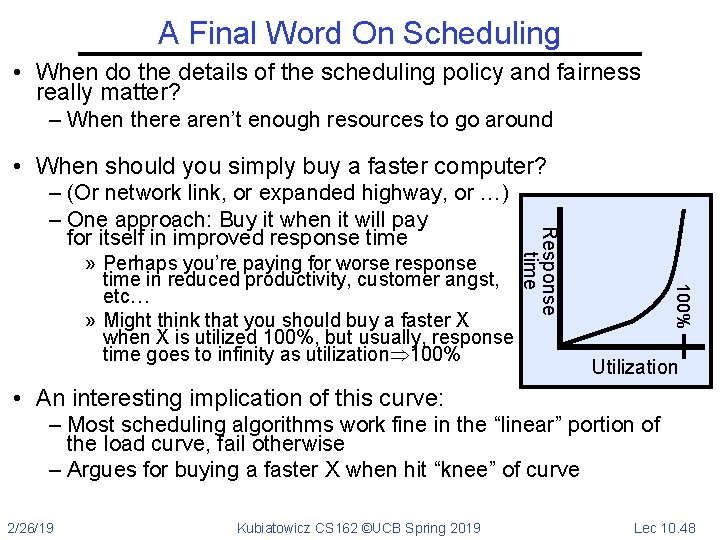
A Final Word On Scheduling • When do the details of the scheduling policy and fairness really matter? – When there aren’t enough resources to go around • When should you simply buy a faster computer? » Perhaps you’re paying for worse response time in reduced productivity, customer angst, etc… » Might think that you should buy a faster X when X is utilized 100%, but usually, response time goes to infinity as utilization 100% Response time – (Or network link, or expanded highway, or …) – One approach: Buy it when it will pay for itself in improved response time Utilization • An interesting implication of this curve: – Most scheduling algorithms work fine in the “linear” portion of the load curve, fail otherwise – Argues for buying a faster X when hit “knee” of curve 2/26/19 Kubiatowicz CS 162 ©UCB Spring 2019 Lec 10. 48

Summary (1 of 2) • Round-Robin Scheduling: – Give each thread a small amount of CPU time when it executes; cycle between all ready threads – Pros: Better for short jobs • Shortest Job First (SJF)/Shortest Remaining Time First (SRTF): – Run whatever job has the least amount of computation to do/least remaining amount of computation to do – Pros: Optimal (average response time) – Cons: Hard to predict future, Unfair • Multi-Level Feedback Scheduling: – Multiple queues of different priorities and scheduling algorithms – Automatic promotion/demotion of process priority in order to approximate SJF/SRTF 2/26/19 Kubiatowicz CS 162 ©UCB Spring 2019 Lec 10. 49

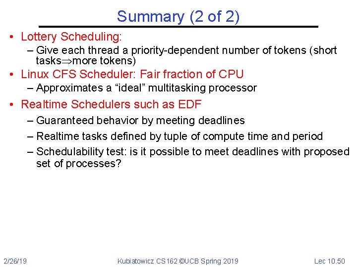
Summary (2 of 2) • Lottery Scheduling: – Give each thread a priority-dependent number of tokens (short tasks more tokens) • Linux CFS Scheduler: Fair fraction of CPU – Approximates a “ideal” multitasking processor • Realtime Schedulers such as EDF – Guaranteed behavior by meeting deadlines – Realtime tasks defined by tuple of compute time and period – Schedulability test: is it possible to meet deadlines with proposed set of processes? 2/26/19 Kubiatowicz CS 162 ©UCB Spring 2019 Lec 10. 50