CS 162 Operating Systems and Systems Programming Lecture

CS 162 Operating Systems and Systems Programming Lecture 8 Thread Scheduling September 30, 2013 Anthony D. Joseph and John Canny http: //inst. eecs. berkeley. edu/~cs 162

Goals for Today • Scheduling Policy goals • Policy Options • Implementation Considerations Note: Some slides and/or pictures in the following are adapted from slides © 2005 Silberschatz, Galvin, and Gagne. Slides courtesy of Anthony D. Joseph, John Kubiatowicz, AJ Shankar, George Necula, Alex Aiken, Eric Brewer, Ras Bodik, Ion Stoica, Doug Tygar, and David Wagner. 9/30/13 Anthony D. Joseph and John Canny CS 162 ©UCB Fall 2013 Lec 8. 2

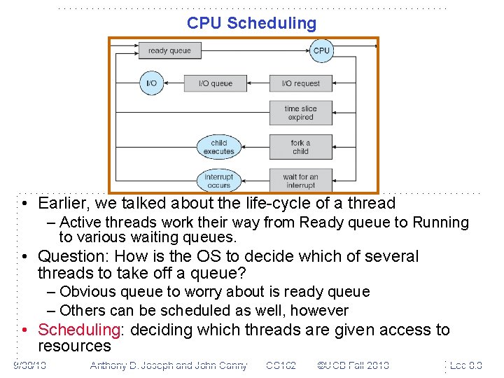
CPU Scheduling • Earlier, we talked about the life-cycle of a thread – Active threads work their way from Ready queue to Running to various waiting queues. • Question: How is the OS to decide which of several threads to take off a queue? – Obvious queue to worry about is ready queue – Others can be scheduled as well, however • Scheduling: deciding which threads are given access to resources 9/30/13 Anthony D. Joseph and John Canny CS 162 ©UCB Fall 2013 Lec 8. 3

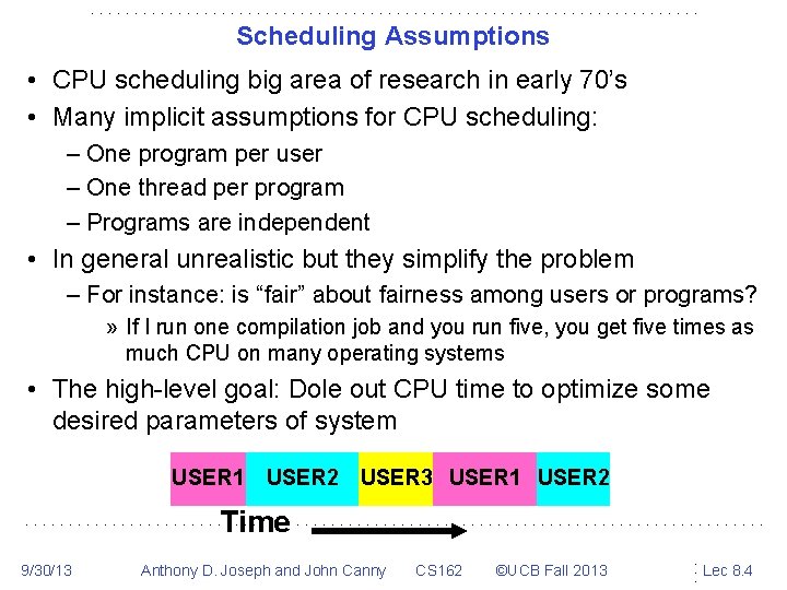
Scheduling Assumptions • CPU scheduling big area of research in early 70’s • Many implicit assumptions for CPU scheduling: – One program per user – One thread per program – Programs are independent • In general unrealistic but they simplify the problem – For instance: is “fair” about fairness among users or programs? » If I run one compilation job and you run five, you get five times as much CPU on many operating systems • The high-level goal: Dole out CPU time to optimize some desired parameters of system USER 1 USER 2 USER 3 USER 1 USER 2 Time 9/30/13 Anthony D. Joseph and John Canny CS 162 ©UCB Fall 2013 Lec 8. 4

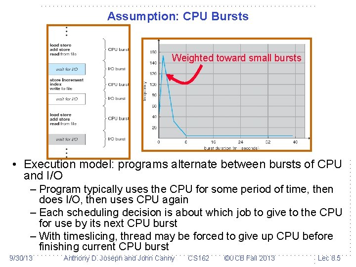
Assumption: CPU Bursts Weighted toward small bursts • Execution model: programs alternate between bursts of CPU and I/O – Program typically uses the CPU for some period of time, then does I/O, then uses CPU again – Each scheduling decision is about which job to give to the CPU for use by its next CPU burst – With timeslicing, thread may be forced to give up CPU before finishing current CPU burst 9/30/13 Anthony D. Joseph and John Canny CS 162 ©UCB Fall 2013 Lec 8. 5

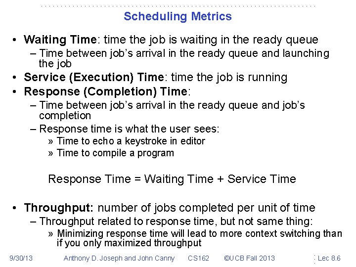
Scheduling Metrics • Waiting Time: time the job is waiting in the ready queue – Time between job’s arrival in the ready queue and launching the job • Service (Execution) Time: time the job is running • Response (Completion) Time: – Time between job’s arrival in the ready queue and job’s completion – Response time is what the user sees: » Time to echo a keystroke in editor » Time to compile a program Response Time = Waiting Time + Service Time • Throughput: number of jobs completed per unit of time – Throughput related to response time, but not same thing: » Minimizing response time will lead to more context switching than if you only maximized throughput 9/30/13 Anthony D. Joseph and John Canny CS 162 ©UCB Fall 2013 Lec 8. 6

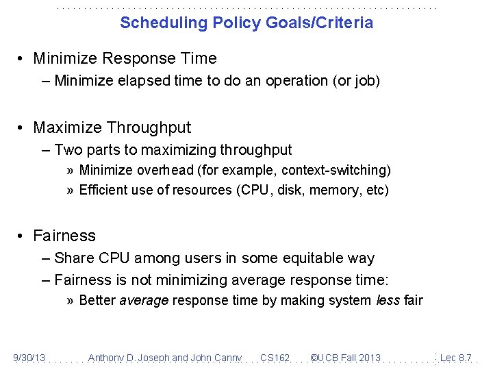
Scheduling Policy Goals/Criteria • Minimize Response Time – Minimize elapsed time to do an operation (or job) • Maximize Throughput – Two parts to maximizing throughput » Minimize overhead (for example, context-switching) » Efficient use of resources (CPU, disk, memory, etc) • Fairness – Share CPU among users in some equitable way – Fairness is not minimizing average response time: » Better average response time by making system less fair 9/30/13 Anthony D. Joseph and John Canny CS 162 ©UCB Fall 2013 Lec 8. 7

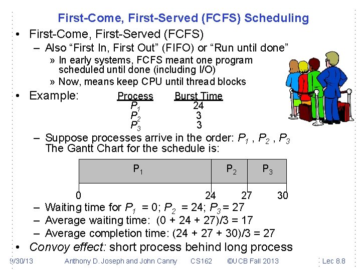
First-Come, First-Served (FCFS) Scheduling • First-Come, First-Served (FCFS) – Also “First In, First Out” (FIFO) or “Run until done” » In early systems, FCFS meant one program scheduled until done (including I/O) » Now, means keep CPU until thread blocks • Example: Process Burst Time P 1 24 P 2 3 P 3 3 – Suppose processes arrive in the order: P 1 , P 2 , P 3 The Gantt Chart for the schedule is: P 1 0 P 2 24 P 3 27 – Waiting time for P 1 = 0; P 2 = 24; P 3 = 27 – Average waiting time: (0 + 24 + 27)/3 = 17 – Average completion time: (24 + 27 + 30)/3 = 27 30 • Convoy effect: short process behind long process 9/30/13 Anthony D. Joseph and John Canny CS 162 ©UCB Fall 2013 Lec 8. 8

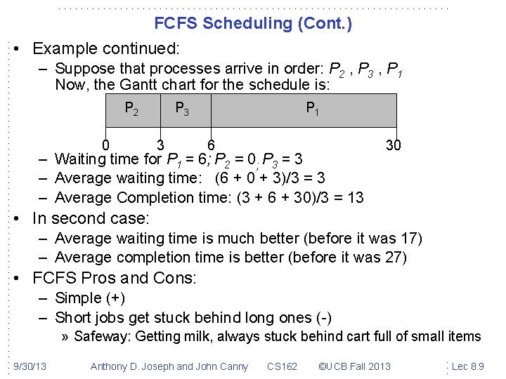
FCFS Scheduling (Cont. ) • Example continued: – Suppose that processes arrive in order: P 2 , P 3 , P 1 Now, the Gantt chart for the schedule is: P 2 0 P 3 3 P 1 6 – Waiting time for P 1 = 6; P 2 = 0; P 3 = 3 – Average waiting time: (6 + 0 + 3)/3 = 3 – Average Completion time: (3 + 6 + 30)/3 = 13 30 • In second case: – Average waiting time is much better (before it was 17) – Average completion time is better (before it was 27) • FCFS Pros and Cons: – Simple (+) – Short jobs get stuck behind long ones (-) » Safeway: Getting milk, always stuck behind cart full of small items 9/30/13 Anthony D. Joseph and John Canny CS 162 ©UCB Fall 2013 Lec 8. 9

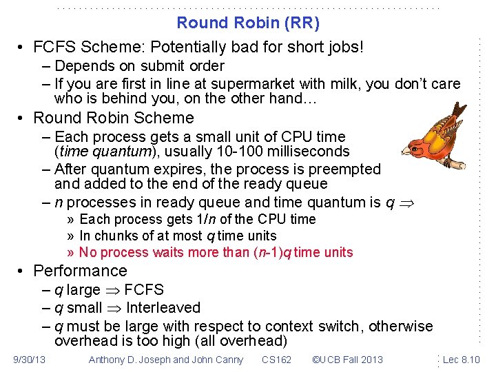
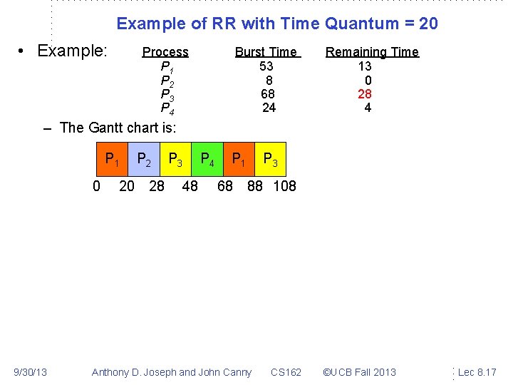
Round Robin (RR) • FCFS Scheme: Potentially bad for short jobs! – Depends on submit order – If you are first in line at supermarket with milk, you don’t care who is behind you, on the other hand… • Round Robin Scheme – Each process gets a small unit of CPU time (time quantum), usually 10 -100 milliseconds – After quantum expires, the process is preempted and added to the end of the ready queue – n processes in ready queue and time quantum is q » Each process gets 1/n of the CPU time » In chunks of at most q time units » No process waits more than (n-1)q time units • Performance – q large FCFS – q small Interleaved – q must be large with respect to context switch, otherwise overhead is too high (all overhead) 9/30/13 Anthony D. Joseph and John Canny CS 162 ©UCB Fall 2013 Lec 8. 10

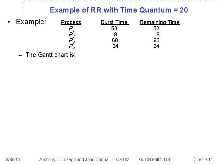
Example of RR with Time Quantum = 20 • Example: Process P 1 P 2 P 3 P 4 Burst Time 53 8 68 24 Remaining Time 53 8 68 24 – The Gantt chart is: 9/30/13 Anthony D. Joseph and John Canny CS 162 ©UCB Fall 2013 Lec 8. 11

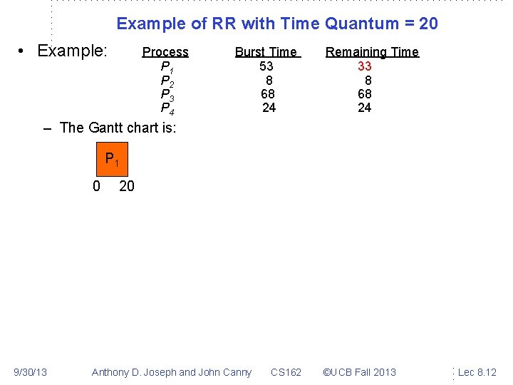
Example of RR with Time Quantum = 20 • Example: Process P 1 P 2 P 3 P 4 Burst Time 53 8 68 24 Remaining Time 33 8 68 24 – The Gantt chart is: P 1 0 9/30/13 20 Anthony D. Joseph and John Canny CS 162 ©UCB Fall 2013 Lec 8. 12

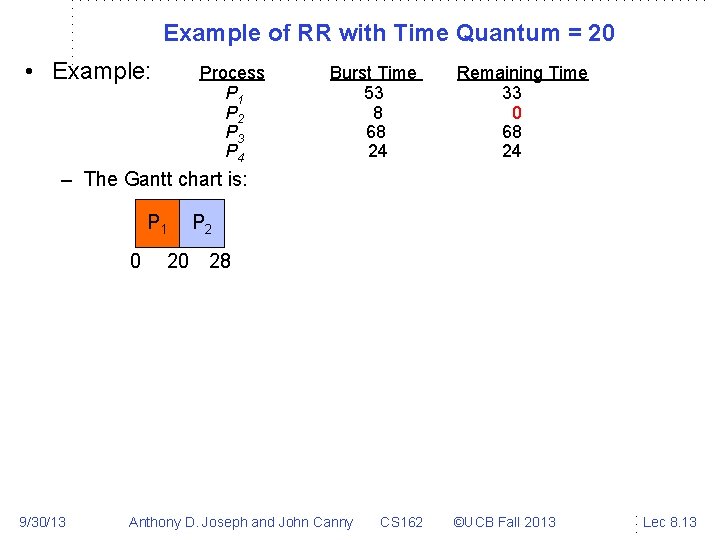
Example of RR with Time Quantum = 20 • Example: Process P 1 P 2 P 3 P 4 Burst Time 53 8 68 24 Remaining Time 33 0 68 24 – The Gantt chart is: P 1 0 9/30/13 P 2 20 28 Anthony D. Joseph and John Canny CS 162 ©UCB Fall 2013 Lec 8. 13

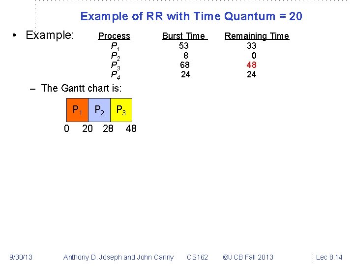
Example of RR with Time Quantum = 20 • Example: Process P 1 P 2 P 3 P 4 Burst Time 53 8 68 24 Remaining Time 33 0 48 24 – The Gantt chart is: P 1 0 9/30/13 P 2 20 28 P 3 48 Anthony D. Joseph and John Canny CS 162 ©UCB Fall 2013 Lec 8. 14

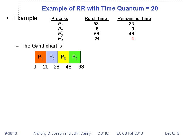
Example of RR with Time Quantum = 20 • Example: Process P 1 P 2 P 3 P 4 Burst Time 53 8 68 24 Remaining Time 33 0 48 4 – The Gantt chart is: P 1 0 9/30/13 P 2 20 28 P 3 48 P 4 68 Anthony D. Joseph and John Canny CS 162 ©UCB Fall 2013 Lec 8. 15

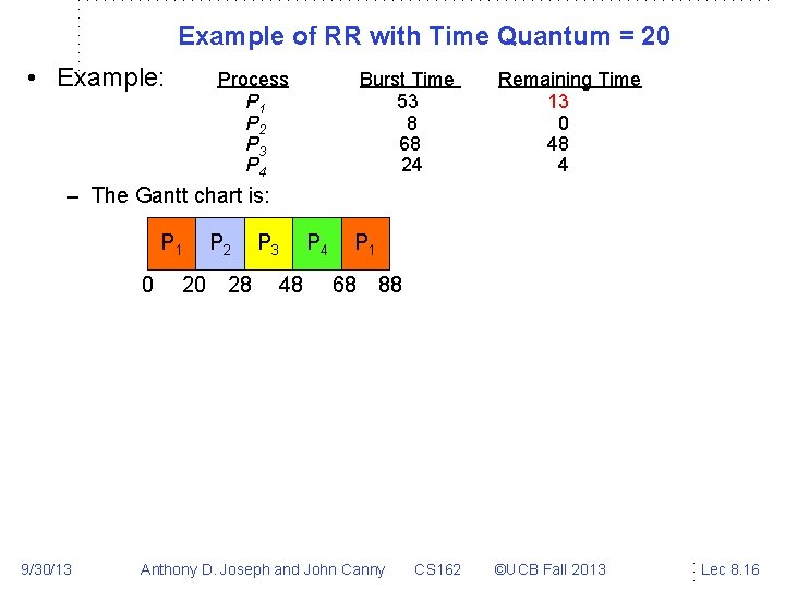
Example of RR with Time Quantum = 20 • Example: Process P 1 P 2 P 3 P 4 Burst Time 53 8 68 24 Remaining Time 13 0 48 4 – The Gantt chart is: P 1 0 9/30/13 P 2 20 28 P 3 48 P 4 P 1 68 88 Anthony D. Joseph and John Canny CS 162 ©UCB Fall 2013 Lec 8. 16

Example of RR with Time Quantum = 20 • Example: Process P 1 P 2 P 3 P 4 Burst Time 53 8 68 24 Remaining Time 13 0 28 4 – The Gantt chart is: P 1 0 9/30/13 P 2 20 28 P 3 48 P 4 P 1 P 3 68 88 108 Anthony D. Joseph and John Canny CS 162 ©UCB Fall 2013 Lec 8. 17

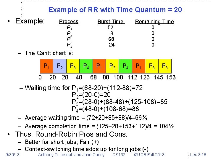
Example of RR with Time Quantum = 20 • Example: Process P 1 P 2 P 3 P 4 Burst Time 53 8 68 24 Remaining Time 0 0 P 1 – The Gantt chart is: P 1 0 P 2 20 28 P 3 48 P 4 P 3 P 3 68 88 108 112 125 145 153 – Waiting time for P 1=(68 -20)+(112 -88)=72 P 2=(20 -0)=20 P 3=(28 -0)+(88 -48)+(125 -108)=85 P 4=(48 -0)+(108 -68)=88 – Average waiting time = (72+20+85+88)/4=66¼ – Average completion time = (125+28+153+112)/4 = 104½ • Thus, Round-Robin Pros and Cons: – Better for short jobs, Fair (+) – Context-switching time adds up for long jobs (-) 9/30/13 Anthony D. Joseph and John Canny CS 162 ©UCB Fall 2013 Lec 8. 18

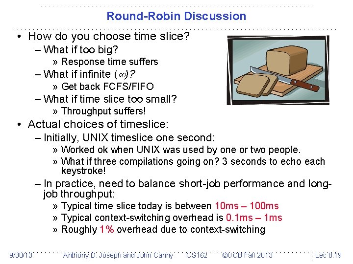
Round-Robin Discussion • How do you choose time slice? – What if too big? » Response time suffers – What if infinite ( )? » Get back FCFS/FIFO – What if time slice too small? » Throughput suffers! • Actual choices of timeslice: – Initially, UNIX timeslice one second: » Worked ok when UNIX was used by one or two people. » What if three compilations going on? 3 seconds to echo each keystroke! – In practice, need to balance short-job performance and longjob throughput: » Typical time slice today is between 10 ms – 100 ms » Typical context-switching overhead is 0. 1 ms – 1 ms » Roughly 1% overhead due to context-switching 9/30/13 Anthony D. Joseph and John Canny CS 162 ©UCB Fall 2013 Lec 8. 19

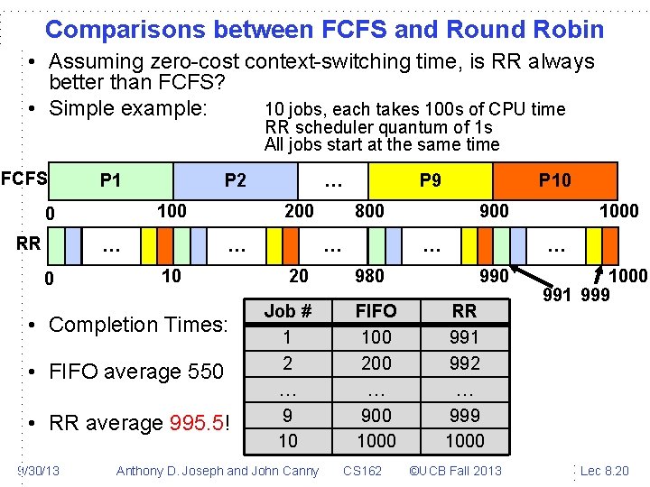
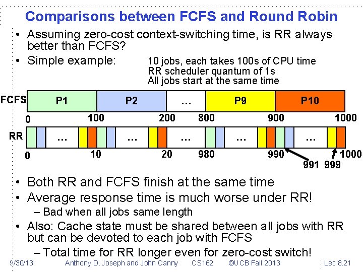
Comparisons between FCFS and Round Robin • Assuming zero-cost context-switching time, is RR always better than FCFS? • Simple example: 10 jobs, each takes 100 s of CPU time RR scheduler quantum of 1 s All jobs start at the same time FCFS P 1 100 0 RR P 2 … 0 200 … 10 • Completion Times: • FIFO average 550 • RR average 995. 5! 9/30/13 … P 9 800 … 20 Job # 1 2 … 9 10 Anthony D. Joseph and John Canny P 10 900 … 980 FIFO 100 200 … 900 1000 CS 162 1000 … 990 RR 991 992 … 999 1000 ©UCB Fall 2013 1000 991 999 Lec 8. 20

Comparisons between FCFS and Round Robin • Assuming zero-cost context-switching time, is RR always better than FCFS? • Simple example: 10 jobs, each takes 100 s of CPU time RR scheduler quantum of 1 s All jobs start at the same time FCFS P 1 100 0 RR P 2 … 0 … 200 … 10 P 9 800 … P 10 900 … 20 980 1000 … 990 1000 991 999 • Both RR and FCFS finish at the same time • Average response time is much worse under RR! – Bad when all jobs same length • Also: Cache state must be shared between all jobs with RR but can be devoted to each job with FCFS – Total time for RR longer even for zero-cost switch! 9/30/13 Anthony D. Joseph and John Canny CS 162 ©UCB Fall 2013 Lec 8. 21

Earlier Example with Different Time Quantum P 2 [8] Best FCFS: 0 P 4 [24] P 1 [53] 8 32 P 3 [68] 85 153 Quantum Best FCFS P 1 32 P 2 0 P 3 85 P 4 8 Average 31¼ Best FCFS 85 8 153 32 69½ Wait Time Completion Time 9/30/13 Anthony D. Joseph and John Canny CS 162 ©UCB Fall 2013 Lec 8. 22

Earlier Example with Different Time Quantum Worst FCFS: P 3 [68] P 1 [53] P 4 [24] 68 0 121 P 2 [8] 145 153 Quantum Best FCFS P 1 32 P 2 0 P 3 85 P 4 8 Average 31¼ Worst FCFS Best FCFS 68 85 145 8 0 153 121 32 83½ 69½ Worst FCFS 121 153 68 145 121¾ Wait Time Completion Time 9/30/13 Anthony D. Joseph and John Canny CS 162 ©UCB Fall 2013 Lec 8. 23

Earlier Example with Different Time Quantum Worst FCFS: P 3 [68] 0 P 1 [53] 68 P 4 [24] 121 P 2 [8] 145 153 Quantum P 1 P 2 P 3 P 4 Average FCFS 32 0 85 8 31¼ P 1 P 2 P 3 P 4 PBest 1 P 3 P 4 P 1 P 3 P 3 P 3 Q=1 84 22 85 57 62 0 8 16 24 32 40 48 56 64 72 80 88 96 104 112 120 128 133 141 149 153 Q=5 82 20 85 58 61¼ Wait Q=8 80 8 85 56 57¼ Time Q = 10 82 10 85 68 61¼ Q = 20 72 20 85 88 66¼ Worst FCFS 68 145 0 121 83½ Best FCFS 85 8 153 32 69½ Q=1 137 30 153 81 100½ Q=5 135 28 153 82 99½ Completion Q=8 133 16 153 80 95½ Time Q = 10 135 18 153 92 99½ Q = 20 125 28 153 112 104½ Worst FCFS 121 153 68 145 121¾ 9/30/13 Anthony D. Joseph and John Canny CS 162 ©UCB Fall 2013 Lec 8. 24

Administrivia • Project #1 code due Tuesday Oct 8 by 11: 59 pm • Midterm #1 is Monday Oct 21 5: 30 -7 pm in 145 Dwinelle (A-L) and 2060 Valley LSB (M-Z) – Closed book, one handwritten page of notes, no calculators – Covers lectures #1 -13, readings, handouts, and projects 1 and 2 – Review session TBA 9/30/13 Anthony D. Joseph and John Canny CS 162 ©UCB Fall 2013 Lec 8. 25

5 min Break 9/30/13 Anthony D. Joseph and John Canny CS 162 ©UCB Fall 2013 Lec 8. 26

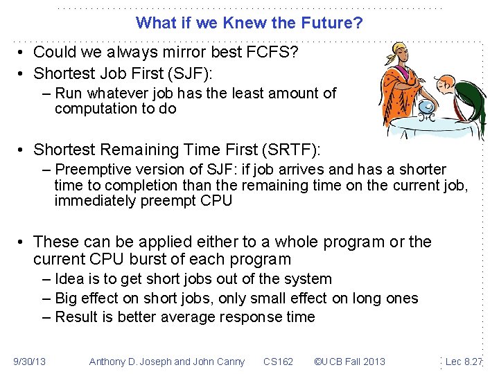
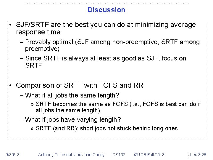
What if we Knew the Future? • Could we always mirror best FCFS? • Shortest Job First (SJF): – Run whatever job has the least amount of computation to do • Shortest Remaining Time First (SRTF): – Preemptive version of SJF: if job arrives and has a shorter time to completion than the remaining time on the current job, immediately preempt CPU • These can be applied either to a whole program or the current CPU burst of each program – Idea is to get short jobs out of the system – Big effect on short jobs, only small effect on long ones – Result is better average response time 9/30/13 Anthony D. Joseph and John Canny CS 162 ©UCB Fall 2013 Lec 8. 27

Discussion • SJF/SRTF are the best you can do at minimizing average response time – Provably optimal (SJF among non-preemptive, SRTF among preemptive) – Since SRTF is always at least as good as SJF, focus on SRTF • Comparison of SRTF with FCFS and RR – What if all jobs the same length? » SRTF becomes the same as FCFS (i. e. , FCFS is best can do if all jobs the same length) – What if jobs have varying length? » SRTF (and RR): short jobs not stuck behind long ones 9/30/13 Anthony D. Joseph and John Canny CS 162 ©UCB Fall 2013 Lec 8. 28

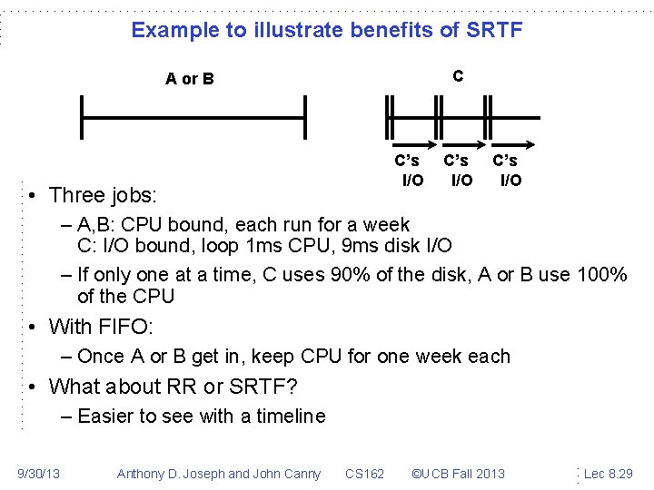
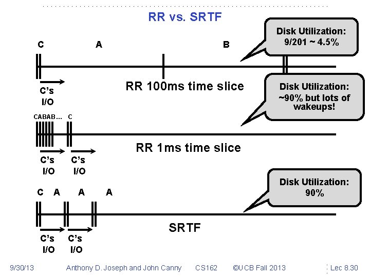
Example to illustrate benefits of SRTF C A or B C’s I/O • Three jobs: C’s I/O – A, B: CPU bound, each run for a week C: I/O bound, loop 1 ms CPU, 9 ms disk I/O – If only one at a time, C uses 90% of the disk, A or B use 100% of the CPU • With FIFO: – Once A or B get in, keep CPU for one week each • What about RR or SRTF? – Easier to see with a timeline 9/30/13 Anthony D. Joseph and John Canny CS 162 ©UCB Fall 2013 Lec 8. 29

RR vs. SRTF C A Disk Utilization: 9/201 ~ 4. 5% C B RR 100 ms time slice C’s I/O Disk C’s Utilization: ~90% I/O but lots of wakeups! CABAB… C RR 1 ms time slice C’s I/O C A C’s I/O 9/30/13 C’s I/O A C’s I/O Disk Utilization: 90% A SRTF Anthony D. Joseph and John Canny CS 162 ©UCB Fall 2013 Lec 8. 30

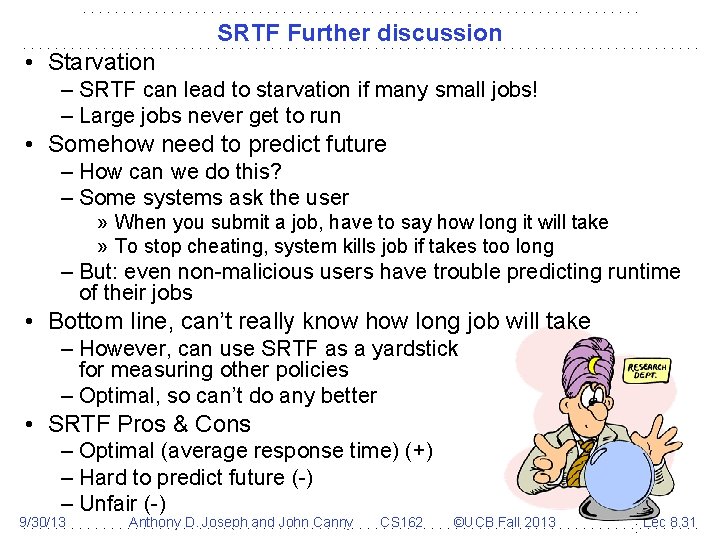
SRTF Further discussion • Starvation – SRTF can lead to starvation if many small jobs! – Large jobs never get to run • Somehow need to predict future – How can we do this? – Some systems ask the user » When you submit a job, have to say how long it will take » To stop cheating, system kills job if takes too long – But: even non-malicious users have trouble predicting runtime of their jobs • Bottom line, can’t really know how long job will take – However, can use SRTF as a yardstick for measuring other policies – Optimal, so can’t do any better • SRTF Pros & Cons – Optimal (average response time) (+) – Hard to predict future (-) – Unfair (-) 9/30/13 Anthony D. Joseph and John Canny CS 162 ©UCB Fall 2013 Lec 8. 31

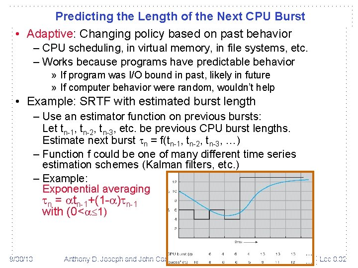
Predicting the Length of the Next CPU Burst • Adaptive: Changing policy based on past behavior – CPU scheduling, in virtual memory, in file systems, etc. – Works because programs have predictable behavior » If program was I/O bound in past, likely in future » If computer behavior were random, wouldn’t help • Example: SRTF with estimated burst length – Use an estimator function on previous bursts: Let tn-1, tn-2, tn-3, etc. be previous CPU burst lengths. Estimate next burst n = f(tn-1, tn-2, tn-3, …) – Function f could be one of many different time series estimation schemes (Kalman filters, etc. ) – Example: Exponential averaging n = tn-1+(1 - ) n-1 with (0< 1) 9/30/13 Anthony D. Joseph and John Canny CS 162 ©UCB Fall 2013 Lec 8. 32

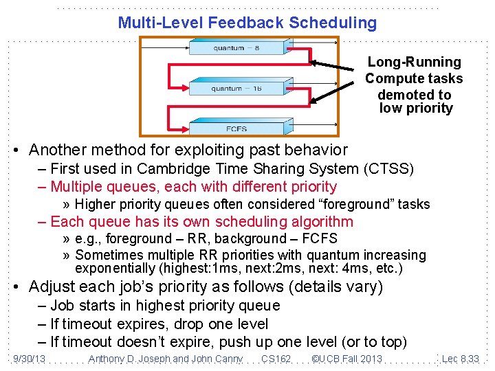
Multi-Level Feedback Scheduling Long-Running Compute tasks demoted to low priority • Another method for exploiting past behavior – First used in Cambridge Time Sharing System (CTSS) – Multiple queues, each with different priority » Higher priority queues often considered “foreground” tasks – Each queue has its own scheduling algorithm » e. g. , foreground – RR, background – FCFS » Sometimes multiple RR priorities with quantum increasing exponentially (highest: 1 ms, next: 2 ms, next: 4 ms, etc. ) • Adjust each job’s priority as follows (details vary) – Job starts in highest priority queue – If timeout expires, drop one level – If timeout doesn’t expire, push up one level (or to top) 9/30/13 Anthony D. Joseph and John Canny CS 162 ©UCB Fall 2013 Lec 8. 33

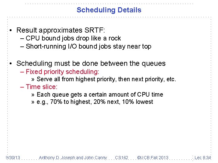
Scheduling Details • Result approximates SRTF: – CPU bound jobs drop like a rock – Short-running I/O bound jobs stay near top • Scheduling must be done between the queues – Fixed priority scheduling: » Serve all from highest priority, then next priority, etc. – Time slice: » Each queue gets a certain amount of CPU time » e. g. , 70% to highest, 20% next, 10% lowest 9/30/13 Anthony D. Joseph and John Canny CS 162 ©UCB Fall 2013 Lec 8. 34

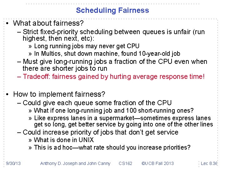
Scheduling Fairness • What about fairness? – Strict fixed-priority scheduling between queues is unfair (run highest, then next, etc): » Long running jobs may never get CPU » In Multics, shut down machine, found 10 -year-old job – Must give long-running jobs a fraction of the CPU even when there are shorter jobs to run – Tradeoff: fairness gained by hurting average response time! • How to implement fairness? – Could give each queue some fraction of the CPU » What if one long-running job and 100 short-running ones? » Like express lanes in a supermarket—sometimes express lanes get so long, get better service by going into one of the other lines – Could increase priority of jobs that don’t get service » What is done in UNIX » This is ad hoc—what rate should you increase priorities? 9/30/13 Anthony D. Joseph and John Canny CS 162 ©UCB Fall 2013 Lec 8. 36

Lottery Scheduling • Yet another alternative: Lottery Scheduling – Give each job some number of lottery tickets – On each time slice, randomly pick a winning ticket – On average, CPU time is proportional to number of tickets given to each job • How to assign tickets? – To approximate SRTF, short running jobs get more, long running jobs get fewer – To avoid starvation, every job gets at least one ticket (everyone makes progress) • Advantage over strict priority scheduling: behaves gracefully as load changes – Adding or deleting a job affects all jobs proportionally, independent of how many tickets each job possesses 9/30/13 Anthony D. Joseph and John Canny CS 162 ©UCB Fall 2013 Lec 8. 37

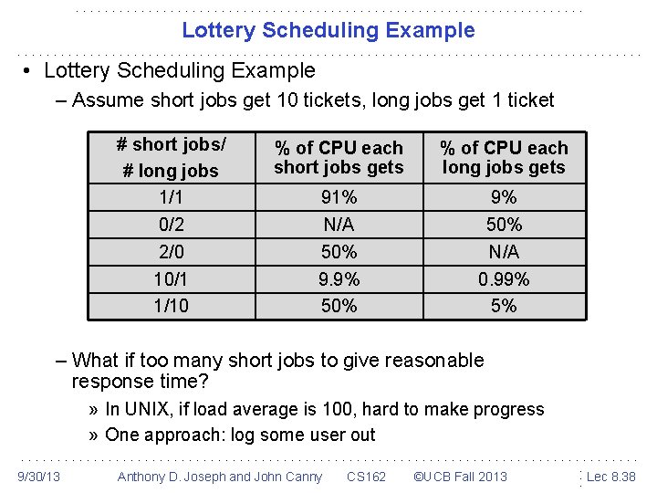
Lottery Scheduling Example • Lottery Scheduling Example – Assume short jobs get 10 tickets, long jobs get 1 ticket # short jobs/ # long jobs 1/1 0/2 2/0 10/1 1/10 % of CPU each short jobs gets % of CPU each long jobs gets 91% N/A 50% 9. 9% 50% N/A 0. 99% 5% – What if too many short jobs to give reasonable response time? » In UNIX, if load average is 100, hard to make progress » One approach: log some user out 9/30/13 Anthony D. Joseph and John Canny CS 162 ©UCB Fall 2013 Lec 8. 38

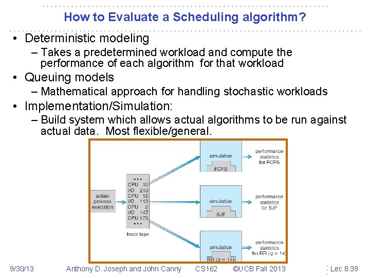
How to Evaluate a Scheduling algorithm? • Deterministic modeling – Takes a predetermined workload and compute the performance of each algorithm for that workload • Queuing models – Mathematical approach for handling stochastic workloads • Implementation/Simulation: – Build system which allows actual algorithms to be run against actual data. Most flexible/general. 9/30/13 Anthony D. Joseph and John Canny CS 162 ©UCB Fall 2013 Lec 8. 39

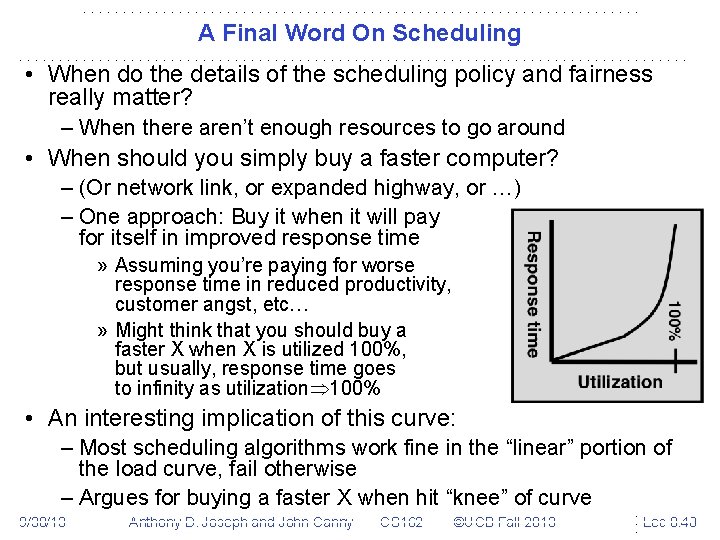
A Final Word On Scheduling • When do the details of the scheduling policy and fairness really matter? – When there aren’t enough resources to go around • When should you simply buy a faster computer? – (Or network link, or expanded highway, or …) – One approach: Buy it when it will pay for itself in improved response time » Assuming you’re paying for worse response time in reduced productivity, customer angst, etc… » Might think that you should buy a faster X when X is utilized 100%, but usually, response time goes to infinity as utilization 100% • An interesting implication of this curve: – Most scheduling algorithms work fine in the “linear” portion of the load curve, fail otherwise – Argues for buying a faster X when hit “knee” of curve 9/30/13 Anthony D. Joseph and John Canny CS 162 ©UCB Fall 2013 Lec 8. 40

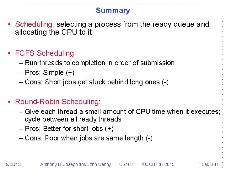
Summary • Scheduling: selecting a process from the ready queue and allocating the CPU to it • FCFS Scheduling: – Run threads to completion in order of submission – Pros: Simple (+) – Cons: Short jobs get stuck behind long ones (-) • Round-Robin Scheduling: – Give each thread a small amount of CPU time when it executes; cycle between all ready threads – Pros: Better for short jobs (+) – Cons: Poor when jobs are same length (-) 9/30/13 Anthony D. Joseph and John Canny CS 162 ©UCB Fall 2013 Lec 8. 41

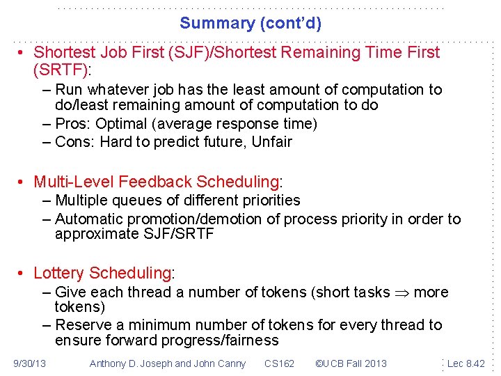
Summary (cont’d) • Shortest Job First (SJF)/Shortest Remaining Time First (SRTF): – Run whatever job has the least amount of computation to do/least remaining amount of computation to do – Pros: Optimal (average response time) – Cons: Hard to predict future, Unfair • Multi-Level Feedback Scheduling: – Multiple queues of different priorities – Automatic promotion/demotion of process priority in order to approximate SJF/SRTF • Lottery Scheduling: – Give each thread a number of tokens (short tasks more tokens) – Reserve a minimum number of tokens for every thread to ensure forward progress/fairness 9/30/13 Anthony D. Joseph and John Canny CS 162 ©UCB Fall 2013 Lec 8. 42