CS 148 Introduction to Computer Graphics and Imaging

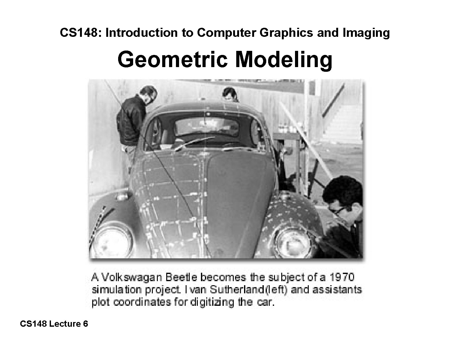
CS 148: Introduction to Computer Graphics and Imaging Geometric Modeling 1/57 CS 148 Lecture 6

Data Structures for Triangle Mesh 2/57 CS 148 Lecture 6

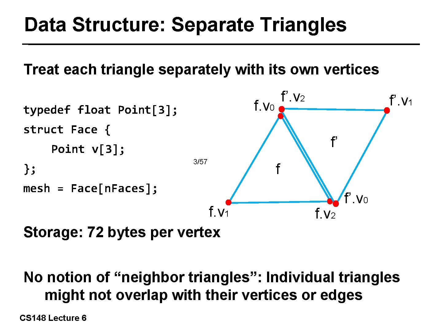
Data Structure: Separate Triangles Treat each triangle separately with its own vertices f’. v 2 f. v 0 typedef float Point[3]; struct Face { f’ Point v[3]; }; f’. v 1 3/57 f mesh = Face[n. Faces]; f. v 1 Storage: 72 bytes per vertex f. v 2 f’. v 0 No notion of “neighbor triangles”: Individual triangles might not overlap with their vertices or edges CS 148 Lecture 6

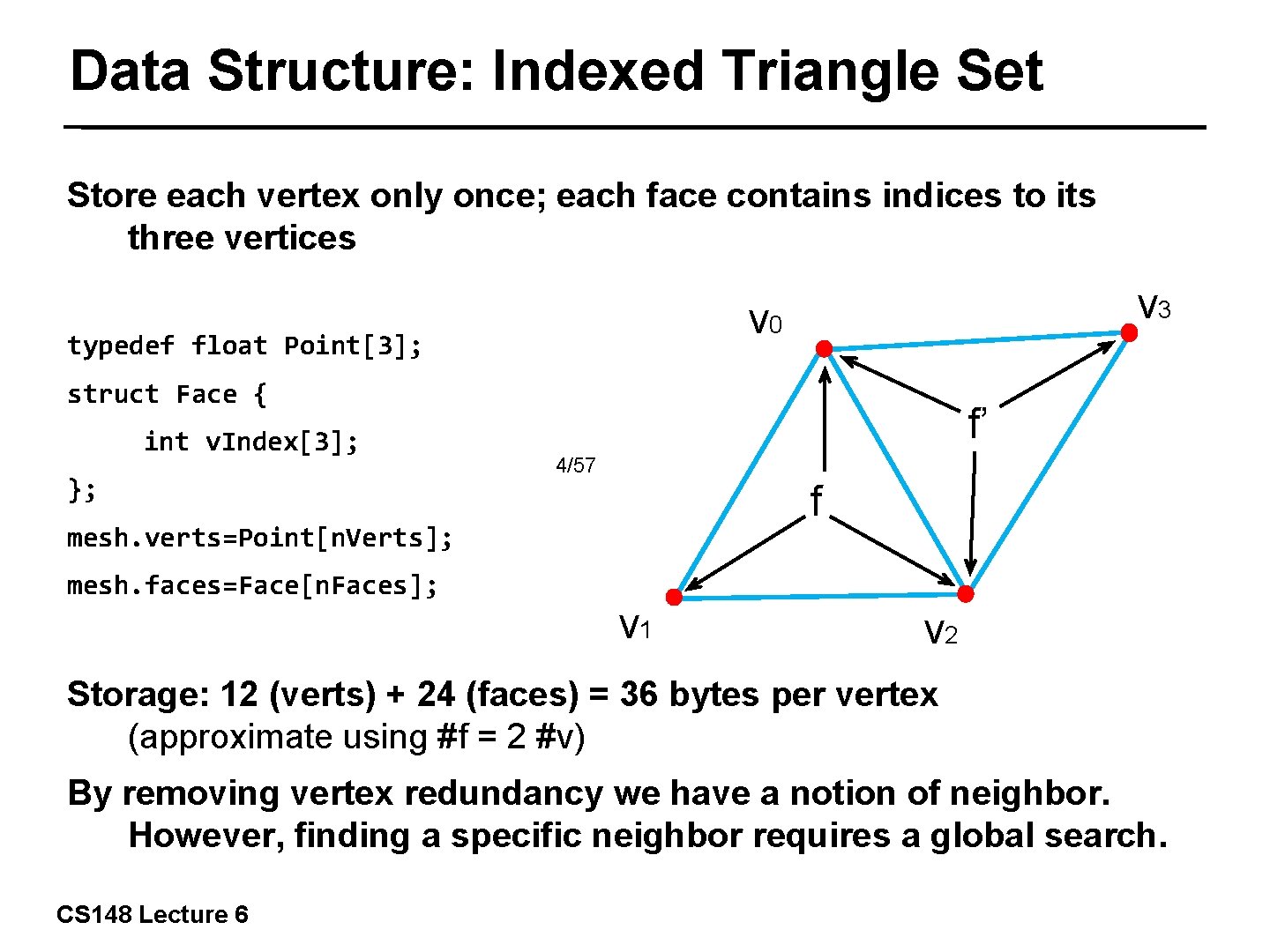
Data Structure: Indexed Triangle Set Store each vertex only once; each face contains indices to its three vertices v 3 v 0 typedef float Point[3]; struct Face { int v. Index[3]; }; f’ 4/57 f mesh. verts=Point[n. Verts]; mesh. faces=Face[n. Faces]; v 1 v 2 Storage: 12 (verts) + 24 (faces) = 36 bytes per vertex (approximate using #f = 2 #v) By removing vertex redundancy we have a notion of neighbor. However, finding a specific neighbor requires a global search. CS 148 Lecture 6

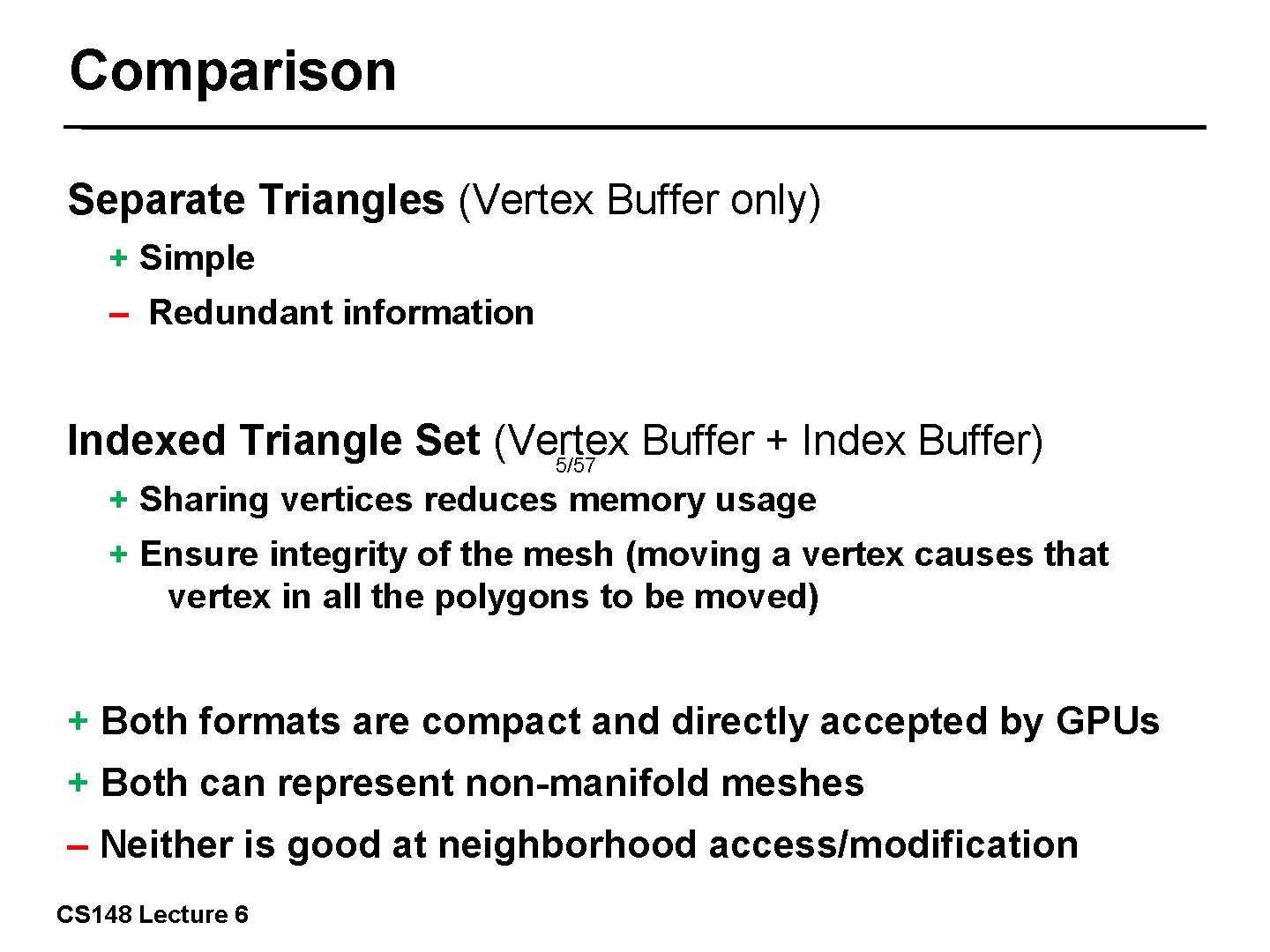
Comparison Separate Triangles (Vertex Buffer only) + Simple – Redundant information Indexed Triangle Set (Vertex Buffer + Index Buffer) 5/57 + Sharing vertices reduces memory usage + Ensure integrity of the mesh (moving a vertex causes that vertex in all the polygons to be moved) + Both formats are compact and directly accepted by GPUs + Both can represent non-manifold meshes – Neither is good at neighborhood access/modification CS 148 Lecture 6

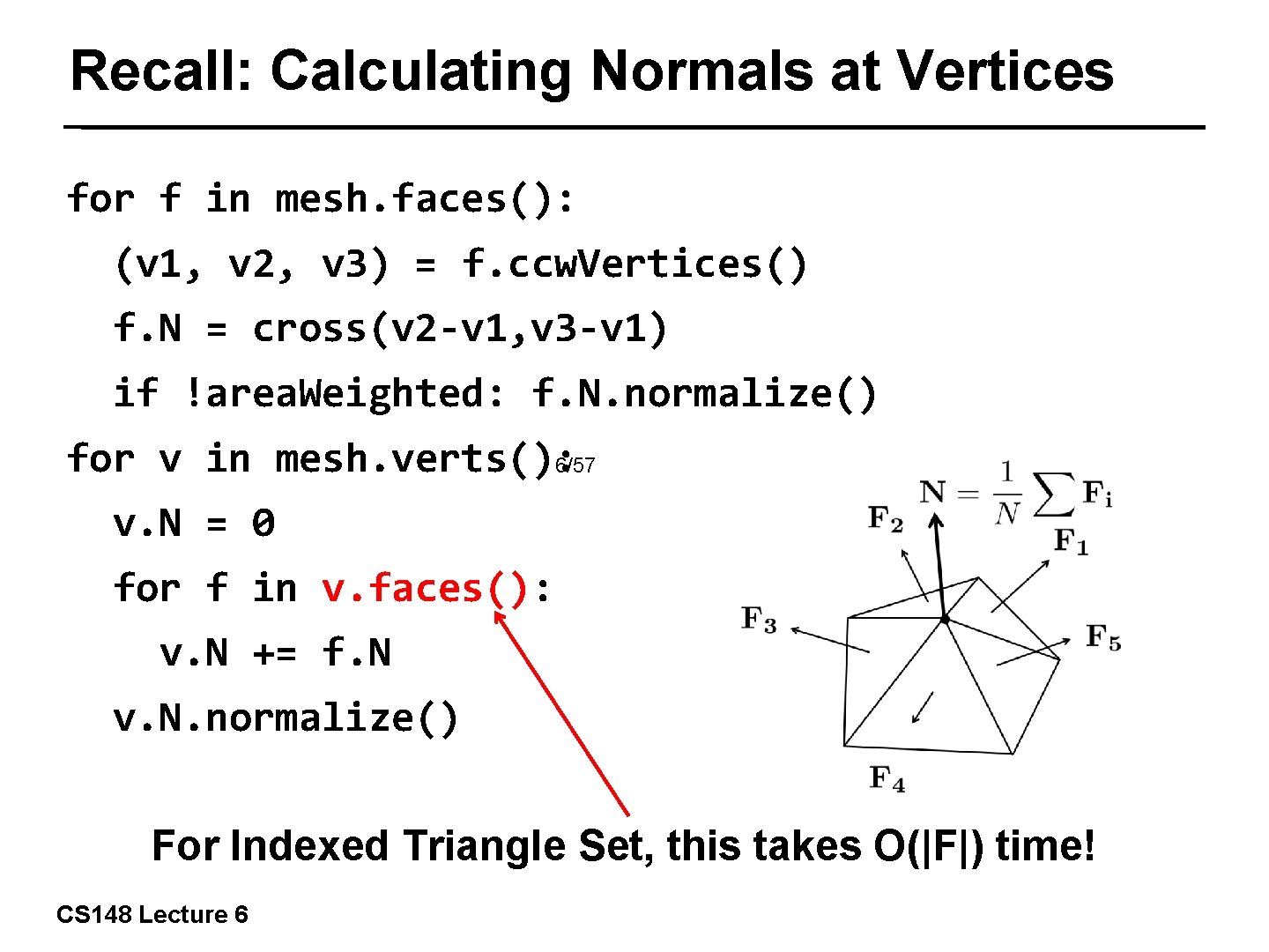
Recall: Calculating Normals at Vertices for f in mesh. faces(): (v 1, v 2, v 3) = f. ccw. Vertices() f. N = cross(v 2 -v 1, v 3 -v 1) if !area. Weighted: f. N. normalize() for v in mesh. verts(): 6/57 v. N = 0 for f in v. faces(): v. N += f. N v. N. normalize() For Indexed Triangle Set, this takes O(|F|) time! CS 148 Lecture 6

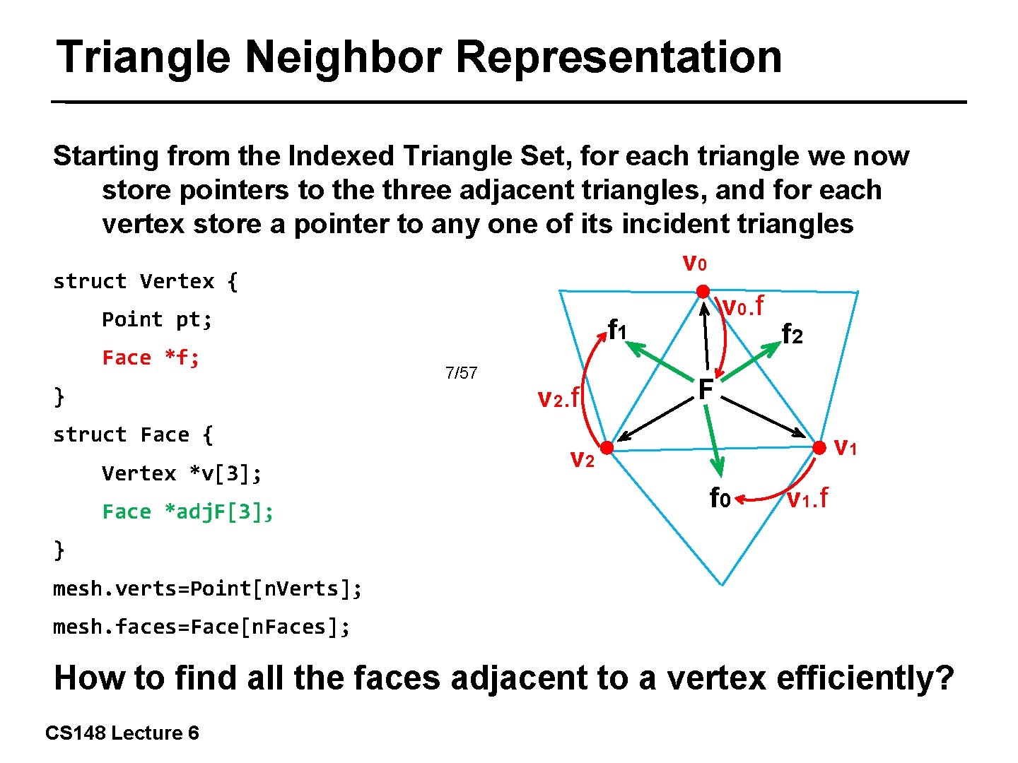
Triangle Neighbor Representation Starting from the Indexed Triangle Set, for each triangle we now store pointers to the three adjacent triangles, and for each vertex store a pointer to any one of its incident triangles v 0 struct Vertex { Point pt; Face *f; } struct Face { Vertex *v[3]; Face *adj. F[3]; v 0. f f 1 7/57 v 2. f f 2 F v 1 v 2 f 0 v 1. f } mesh. verts=Point[n. Verts]; mesh. faces=Face[n. Faces]; How to find all the faces adjacent to a vertex efficiently? CS 148 Lecture 6

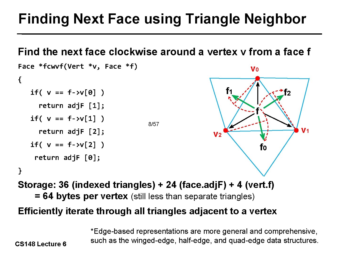
Finding Next Face using Triangle Neighbor Find the next face clockwise around a vertex v from a face f Face *fcwvf(Vert *v, Face *f) v 0 { f 1 if( v == f->v[0] ) return adj. F [1]; if( v == f->v[1] ) return adj. F [2]; if( v == f->v[2] ) f 2 f 8/57 v 1 v 2 f 0 return adj. F [0]; } Storage: 36 (indexed triangles) + 24 (face. adj. F) + 4 (vert. f) = 64 bytes per vertex (still less than separate triangles) Efficiently iterate through all triangles adjacent to a vertex CS 148 Lecture 6 *Edge-based representations are more general and comprehensive, such as the winged-edge, half-edge, and quad-edge data structures.

Subdivision 9/57 CS 148 Lecture 6

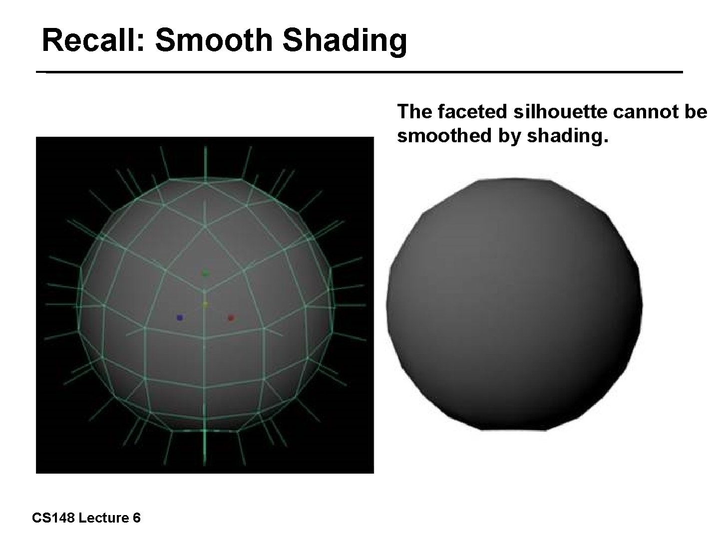
Recall: Smooth Shading The faceted silhouette cannot be smoothed by shading. 10/57 CS 148 Lecture 6

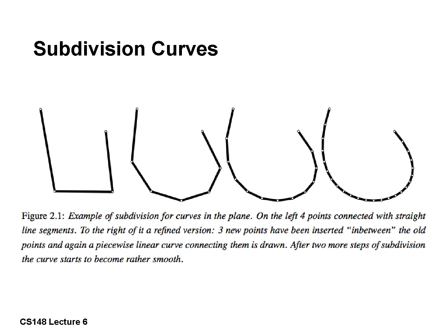
Subdivision Curves 11/57 CS 148 Lecture 6

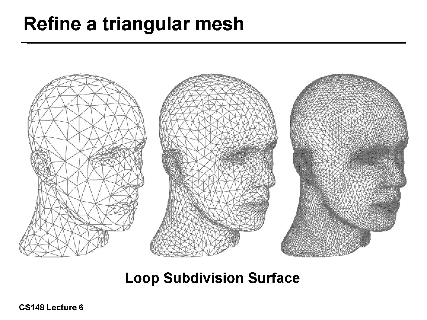
Subdivision Surfaces There exists smooth limit surfaces associated with a given input mesh ￭ The exact smooth limit surface depends on the subdivision algorithm used We define a refinement operation, that takes a coarse input 12/57 mesh and generates a finer output mesh that is closer to the limit surface ￭ ￭ If we apply this refinement process infinitely, we will exactly achieve the target limit surface However, after just a few levels of refinement, any additional changes will be visually indistinguishable CS 148 Lecture 6

Refine a triangular mesh 13/57 Loop Subdivision Surface CS 148 Lecture 6

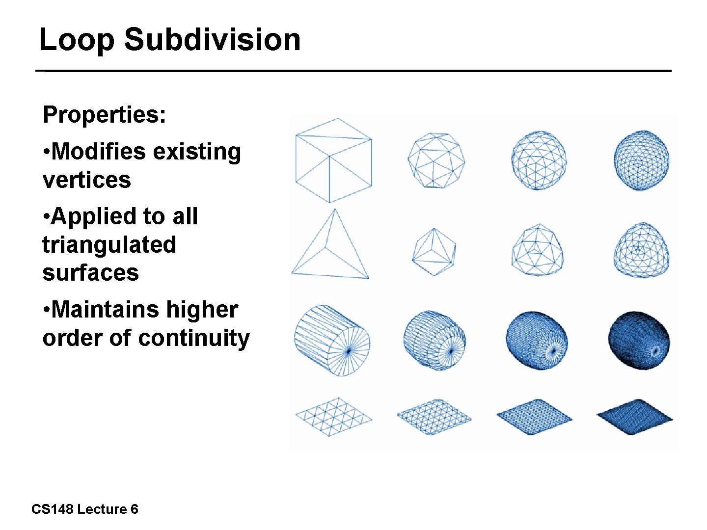
Loop Subdivision Properties: • Modifies existing vertices • Applied to all triangulated surfaces • Maintains higher order of continuity CS 148 Lecture 6 14/57

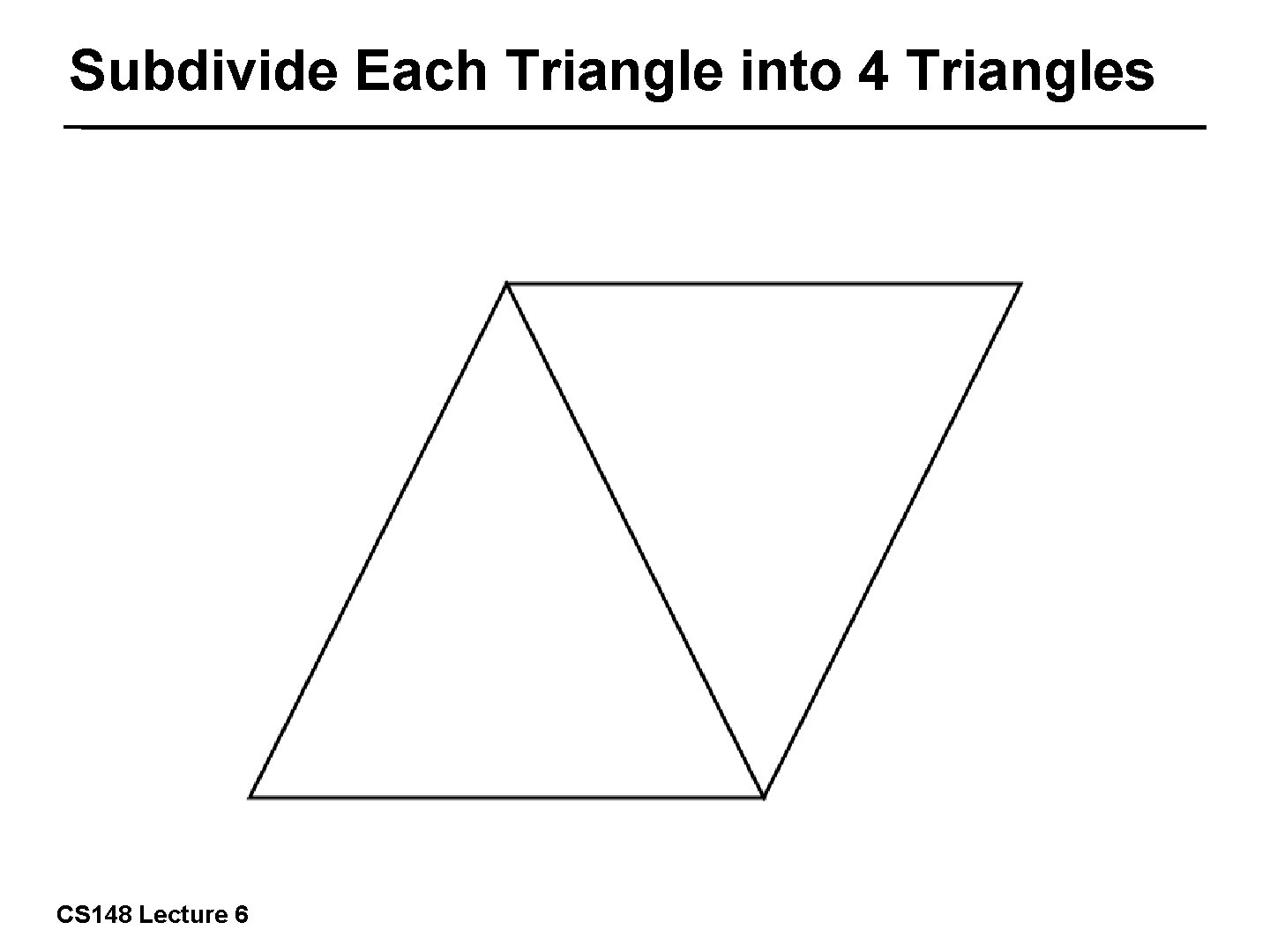
Subdivide Each Triangle into 4 Triangles 15/57 CS 148 Lecture 6

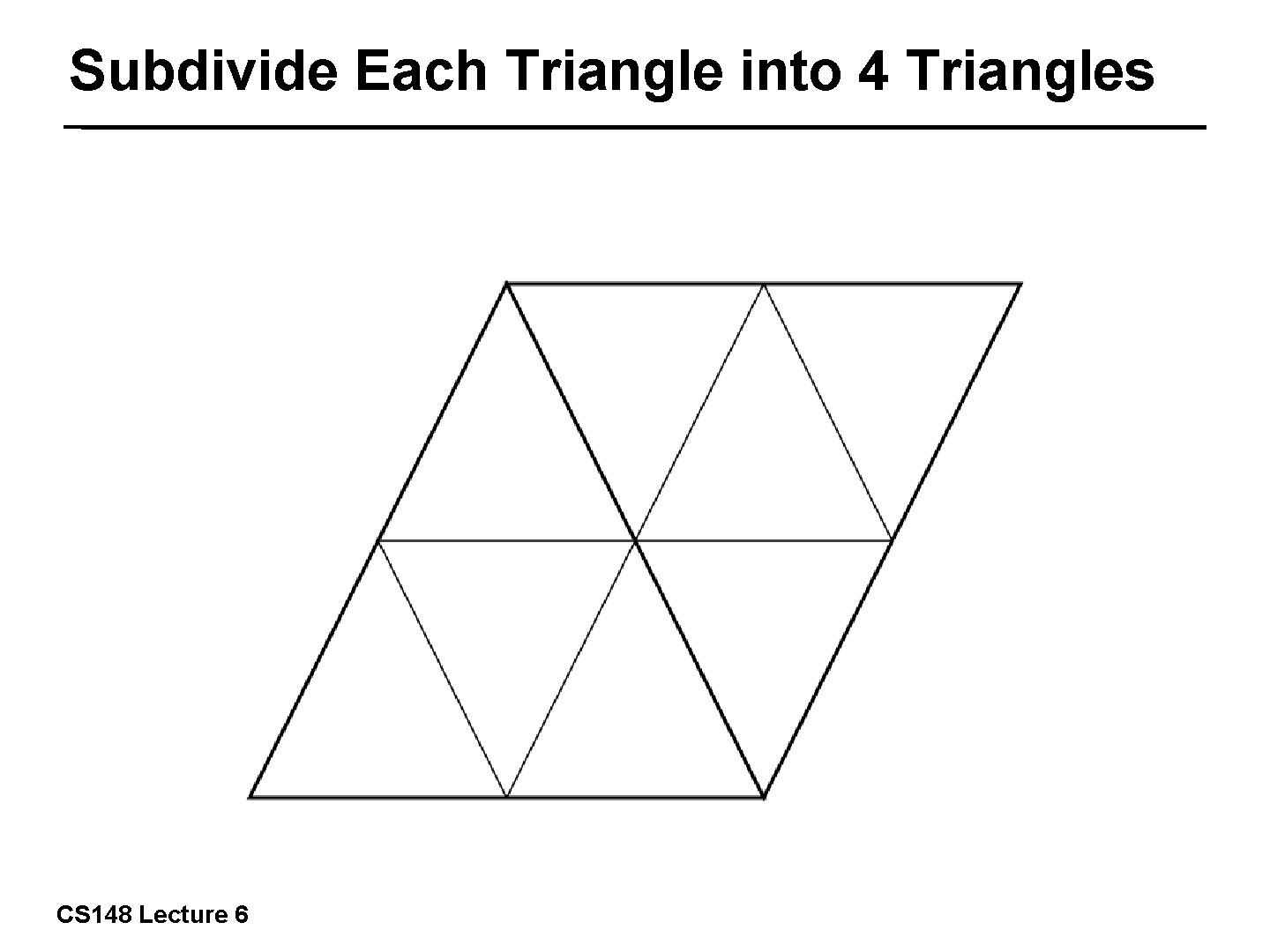
Subdivide Each Triangle into 4 Triangles 16/57 CS 148 Lecture 6

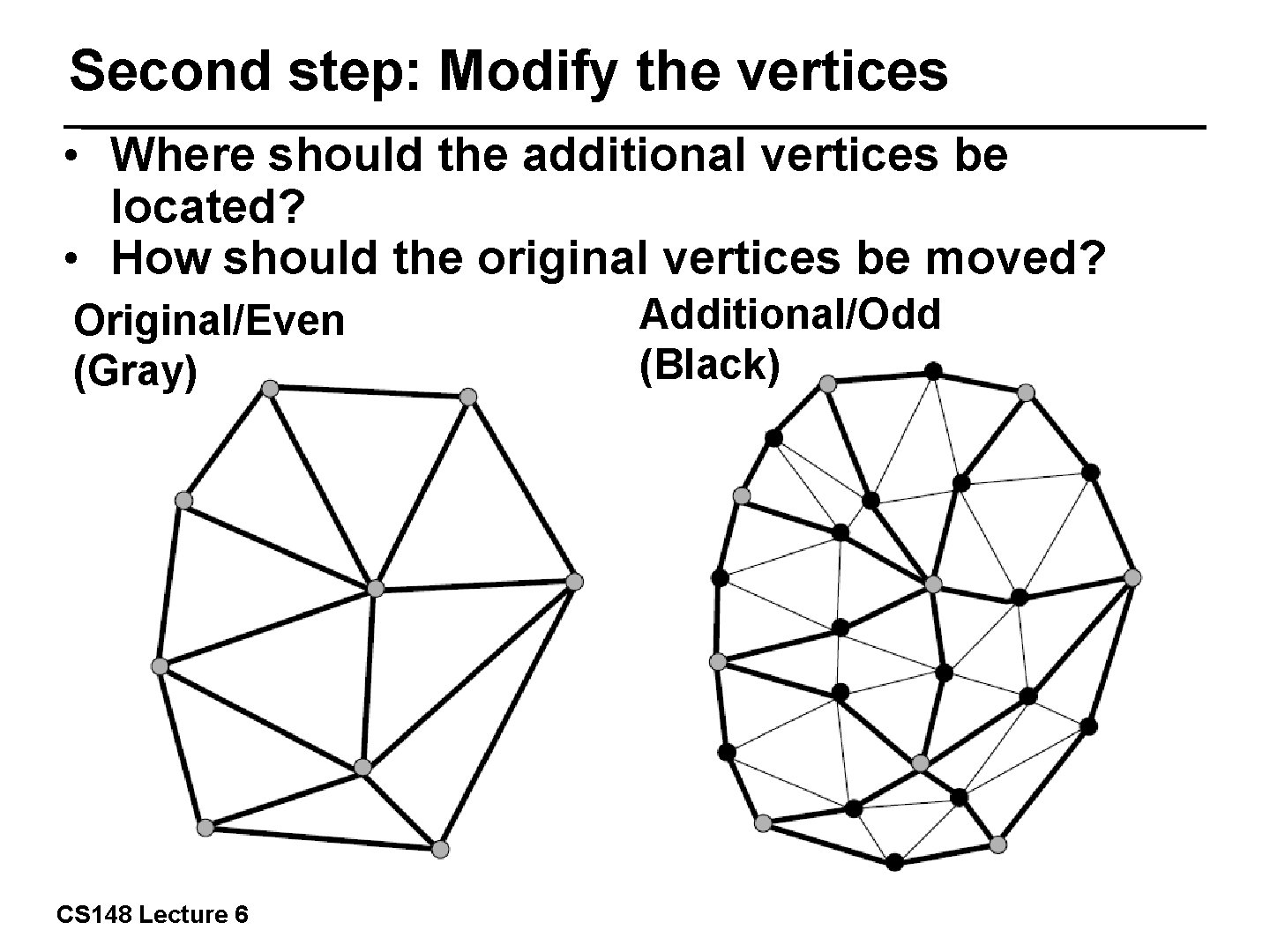
Second step: Modify the vertices • Where should the additional vertices be located? • How should the original vertices be moved? Additional/Odd (Black) Original/Even (Gray) 17/57 CS 148 Lecture 6

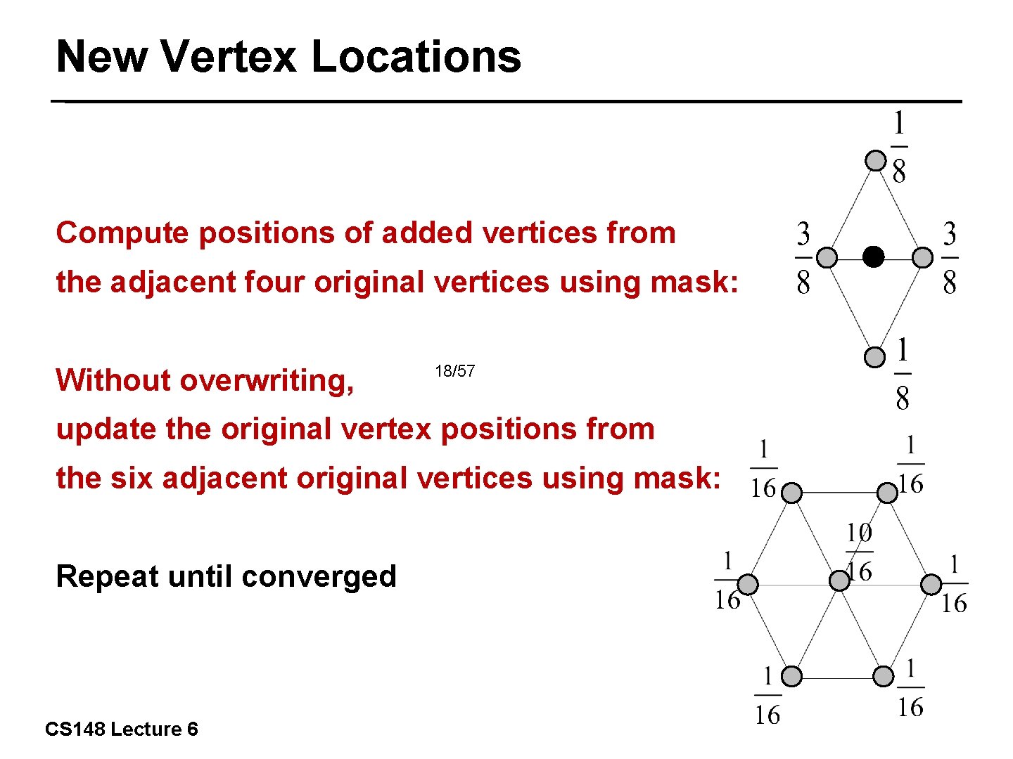
New Vertex Locations Compute positions of added vertices from the adjacent four original vertices using mask: Without overwriting, 18/57 update the original vertex positions from the six adjacent original vertices using mask: Repeat until converged CS 148 Lecture 6

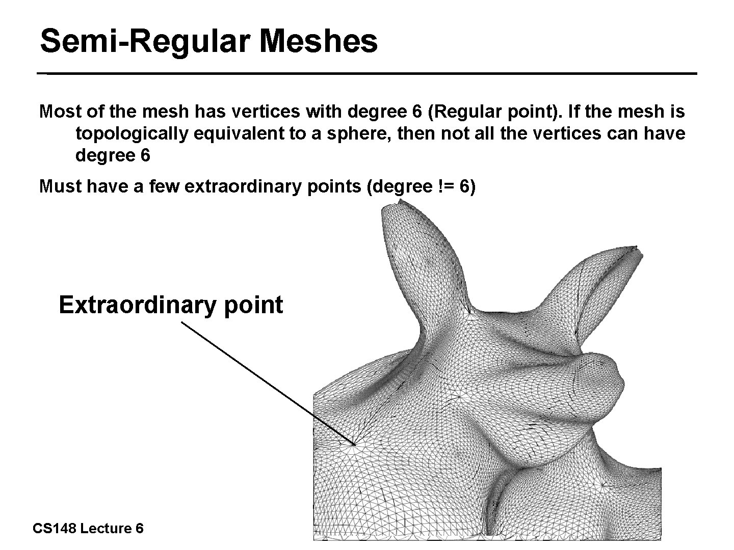
Semi-Regular Meshes Most of the mesh has vertices with degree 6 (Regular point). If the mesh is topologically equivalent to a sphere, then not all the vertices can have degree 6 Must have a few extraordinary points (degree != 6) 19/57 Extraordinary point CS 148 Lecture 6

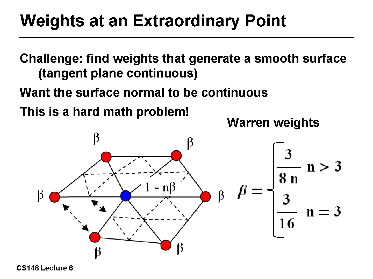
Weights at an Extraordinary Point Challenge: find weights that generate a smooth surface (tangent plane continuous) Want the surface normal to be continuous This is a hard math problem! 20/57 CS 148 Lecture 6 Warren weights

Example mesh 21/57 CS 148 Lecture 6

Example Add vertices 22/57 CS 148 Lecture 6

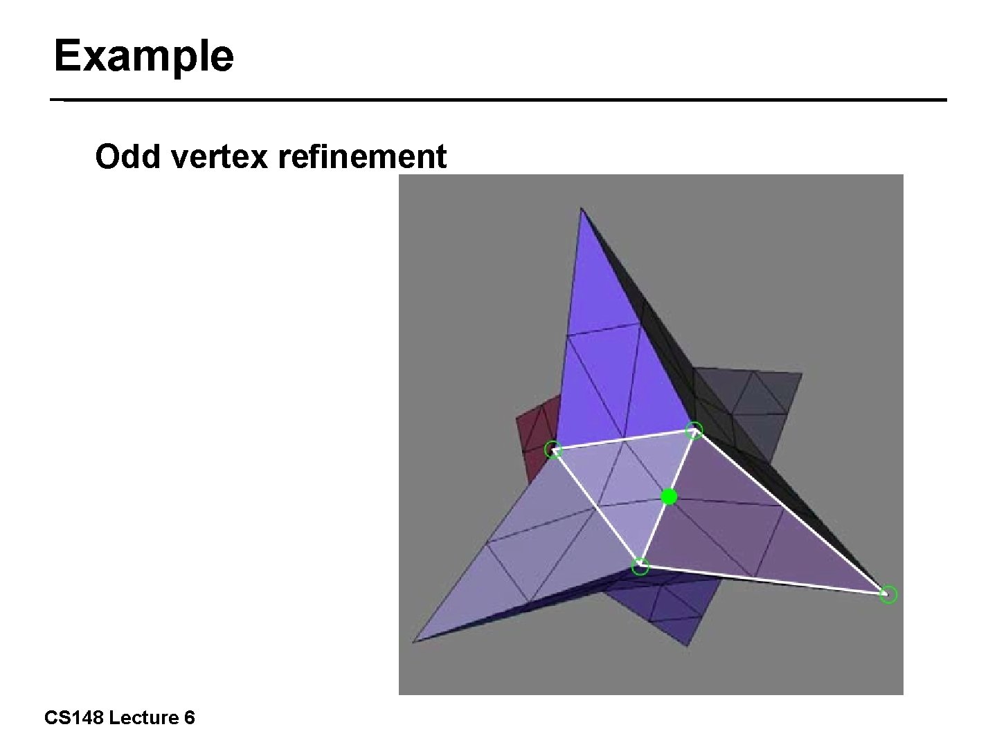
Example Odd vertex refinement 23/57 CS 148 Lecture 6

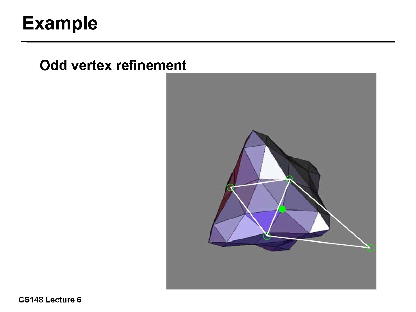
Example Odd vertex refinement 24/57 CS 148 Lecture 6

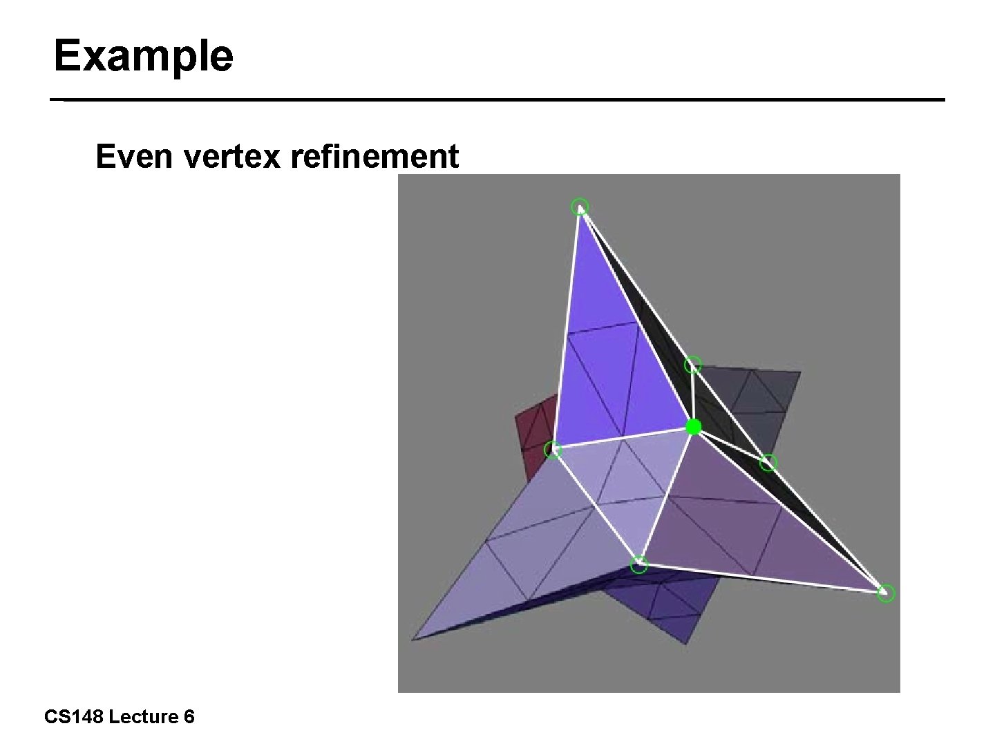
Example Even vertex refinement 25/57 CS 148 Lecture 6

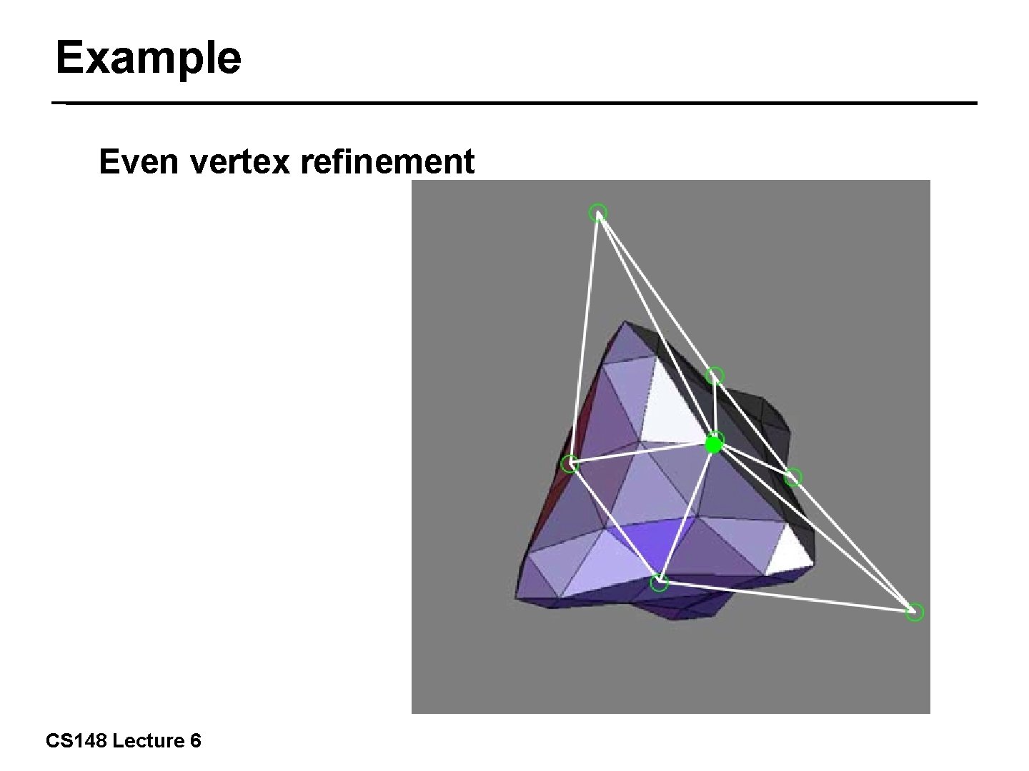
Example Even vertex refinement 26/57 CS 148 Lecture 6

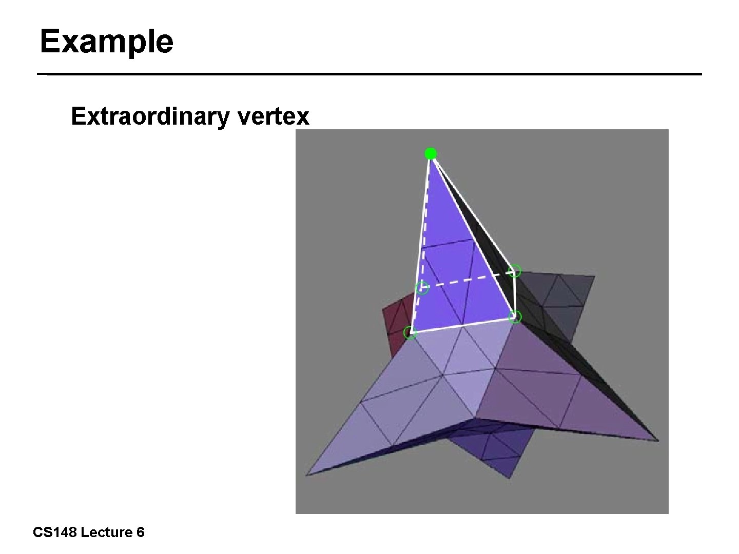
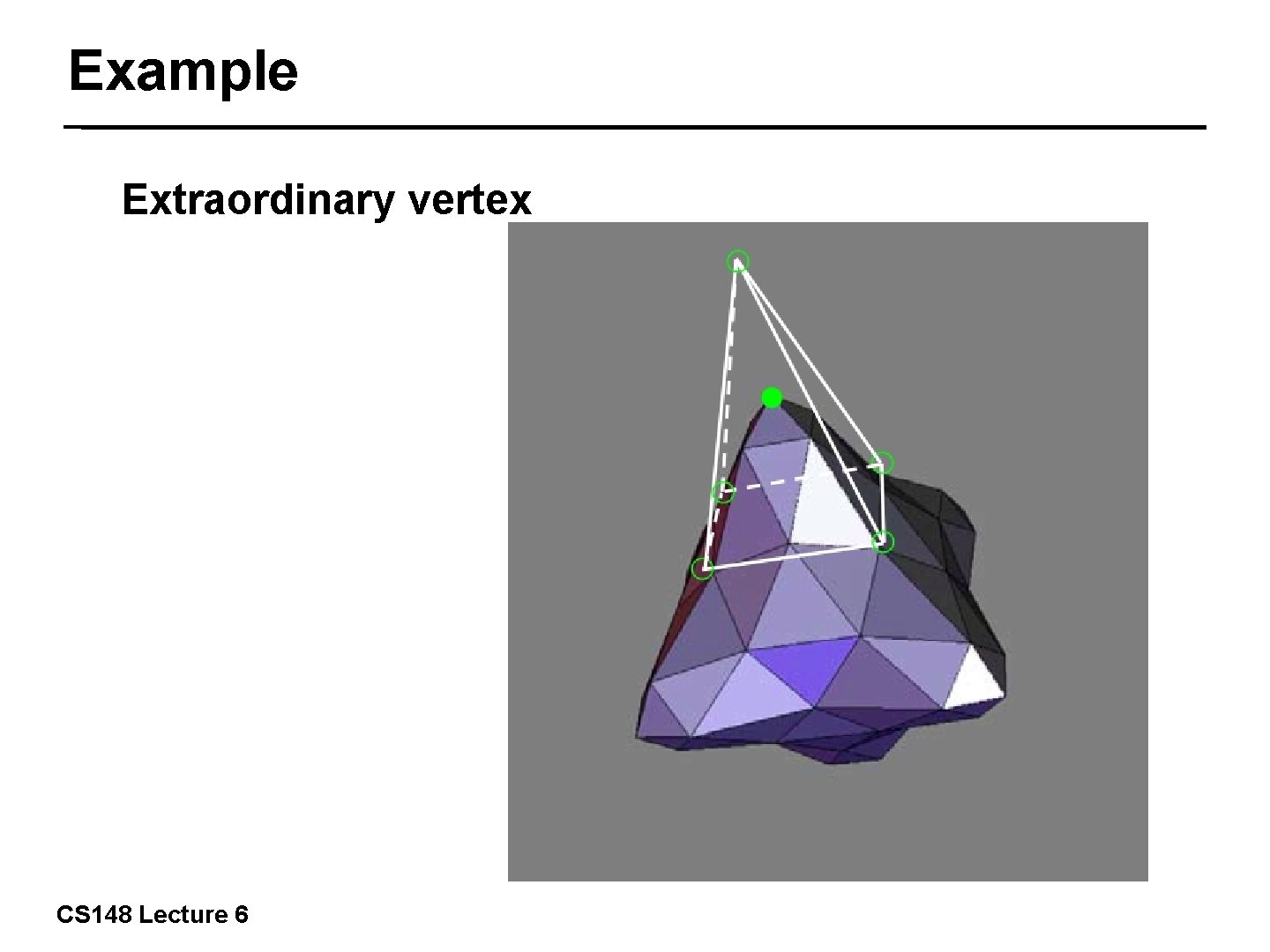
Example Extraordinary vertex 27/57 CS 148 Lecture 6

Example Extraordinary vertex 28/57 CS 148 Lecture 6

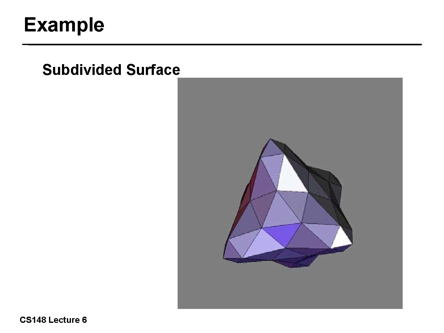
Example Subdivided Surface 29/57 CS 148 Lecture 6

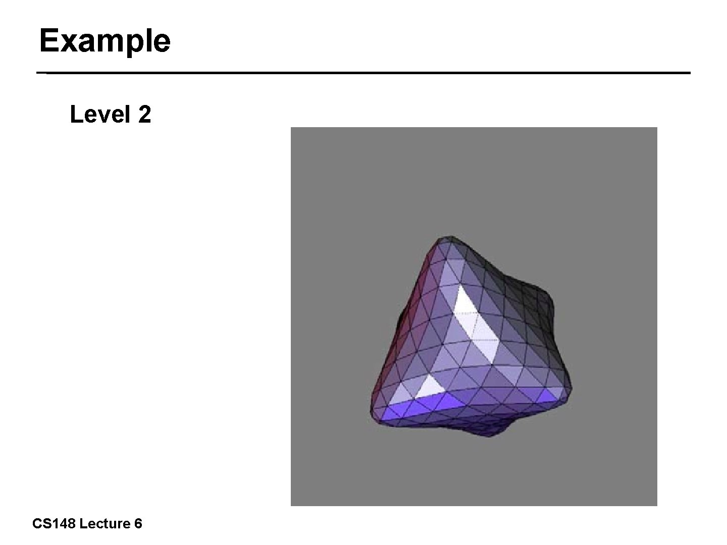
Example Level 2 30/57 CS 148 Lecture 6

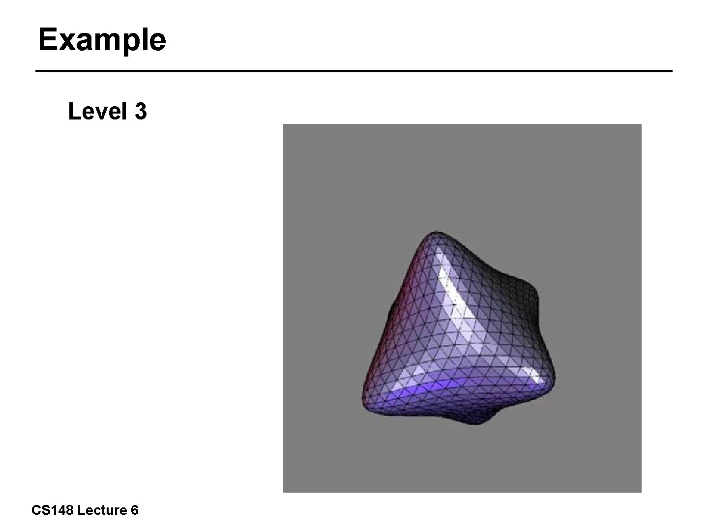
Example Level 3 31/57 CS 148 Lecture 6

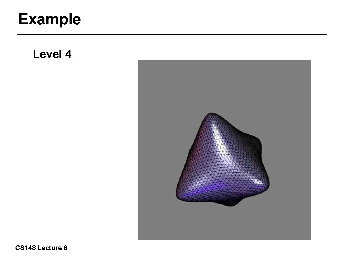
Example Level 4 32/57 CS 148 Lecture 6

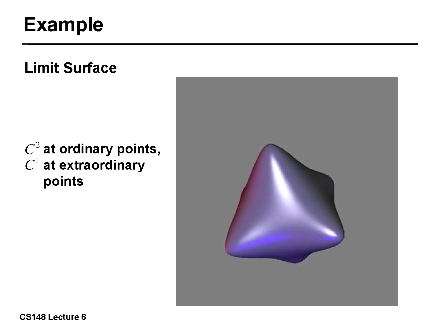
Example Limit Surface at ordinary points, at extraordinary points CS 148 Lecture 6 33/57

Mesh Generation 34/57 CS 148 Lecture 6

Marching Cubes Polygonization ￭ Convert implicit surface to polygonal mesh ￭ Render the polygons as before Two steps 35/57 ￭ Partition space into cells ￭ Fit a polygon to the surface in each cell Gives a piecewise linear approximation of the surface in each cell CS 148 Lecture 6

Cell polygonization Need to find the cells that actually intersect the surface A simple method is: exhaustive enumeration ￭ Divide all of space into a regular grid ￭ Traverse all cells, and polygonize the cells that contain the surface CS 148 Lecture 6 36/57

Surface vertices Determine where the surface intersects the cell edges ￭ 1 st option: Linearly interpolate function value from cell vertices to approximate (function might not be linear) ￭ 2 nd option: Numerically find the zero 37/57 Either will work, but option 2 can be significantly more expensive CS 148 Lecture 6

Surface vertices Linearly interpolate function value from cell vertices to approximate the surface 38/57 CS 148 Lecture 6

Surface polygons Given the vertices of our final polygonal surface, find the polygon faces of the surface Solution: There are only a finite number of options, defined by the configurations of inside/outside of the cell’s vertices 39/57 CS 148 Lecture 6

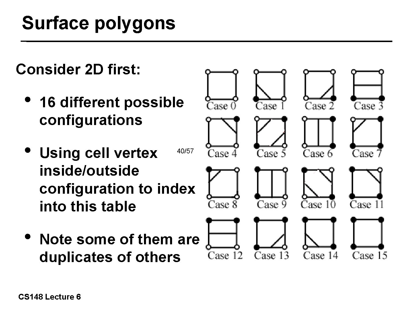
Surface polygons Consider 2 D first: • 16 different possible configurations • Using cell vertex inside/outside configuration to index into this table • Note some of them are duplicates of others 40/57 CS 148 Lecture 6

Surface polygons Result: 41/57 CS 148 Lecture 6

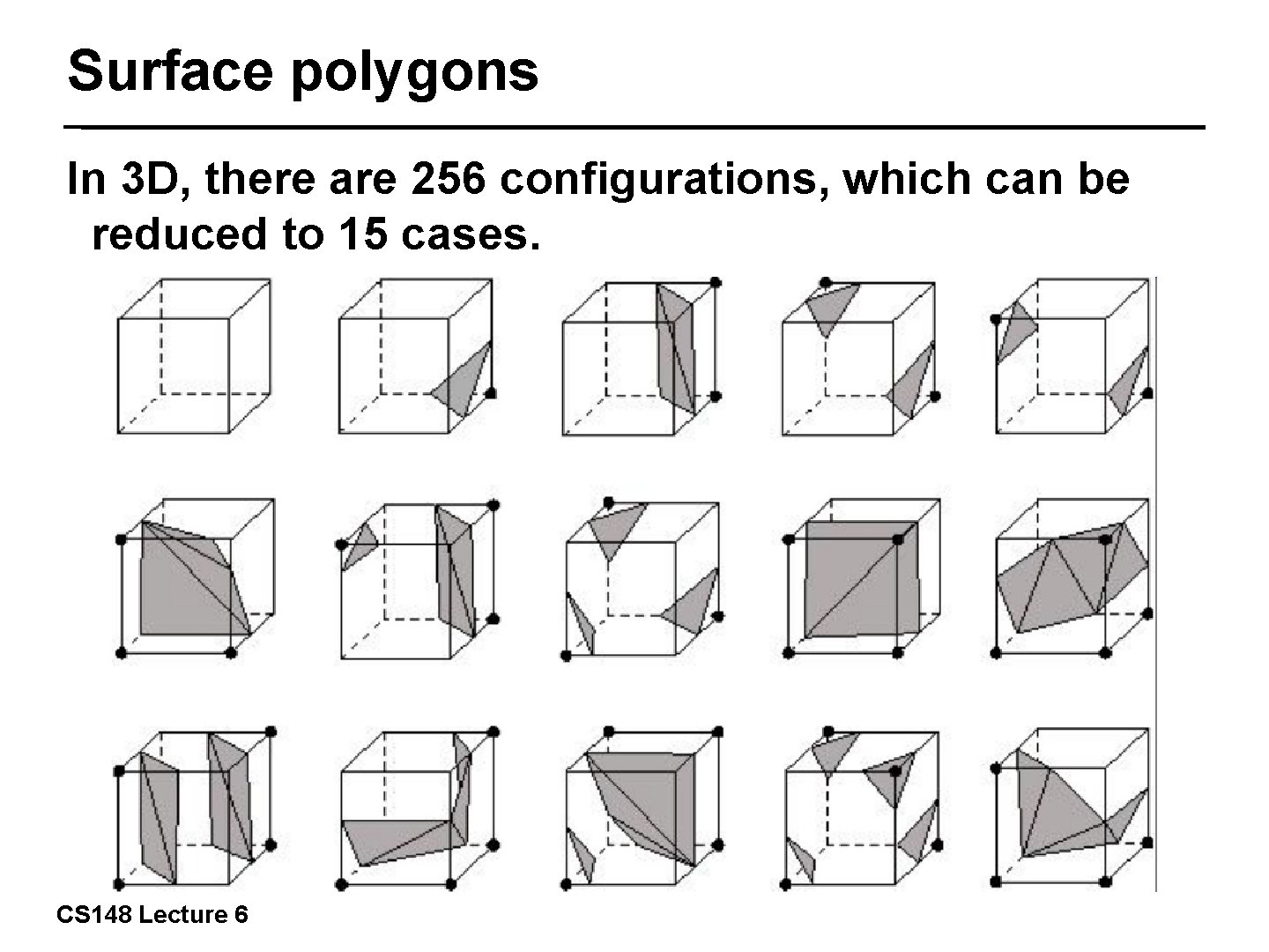
Surface polygons In 3 D, there are 256 configurations, which can be reduced to 15 cases. 42/57 CS 148 Lecture 6

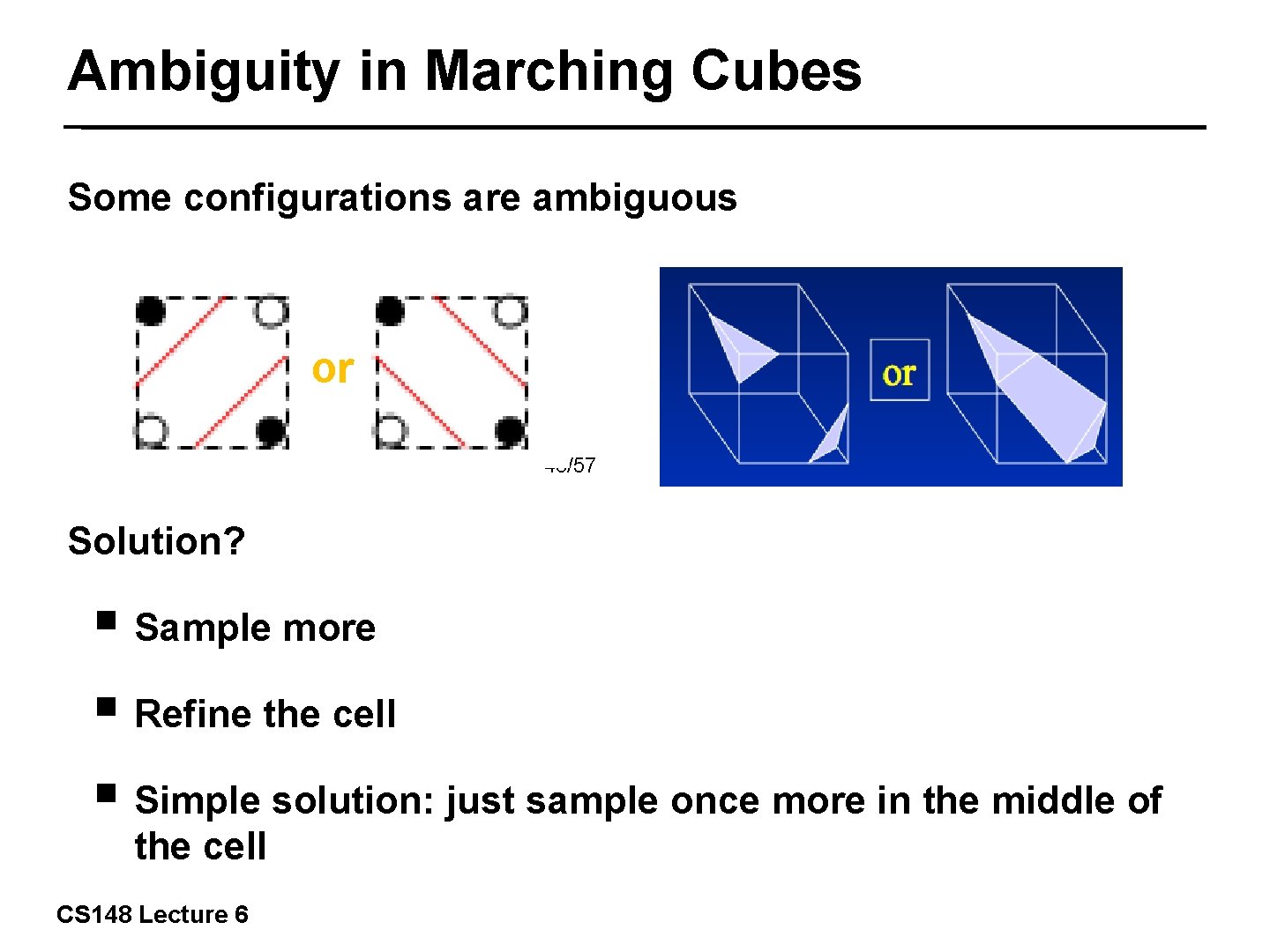
Ambiguity in Marching Cubes Some configurations are ambiguous or 43/57 Solution? ￭ Sample more ￭ Refine the cell ￭ Simple solution: just sample once more in the middle of the cell CS 148 Lecture 6

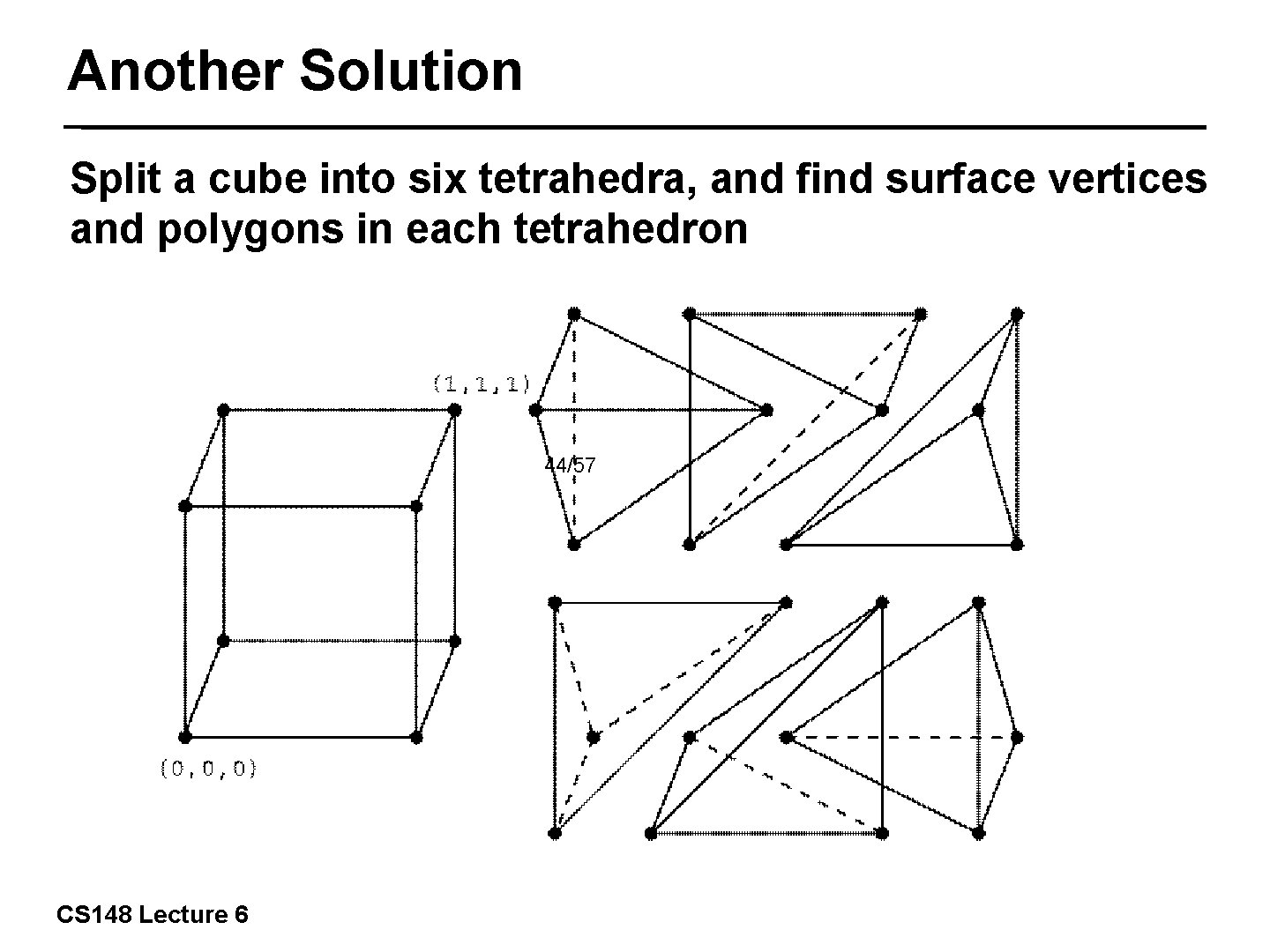
Another Solution Split a cube into six tetrahedra, and find surface vertices and polygons in each tetrahedron 44/57 CS 148 Lecture 6

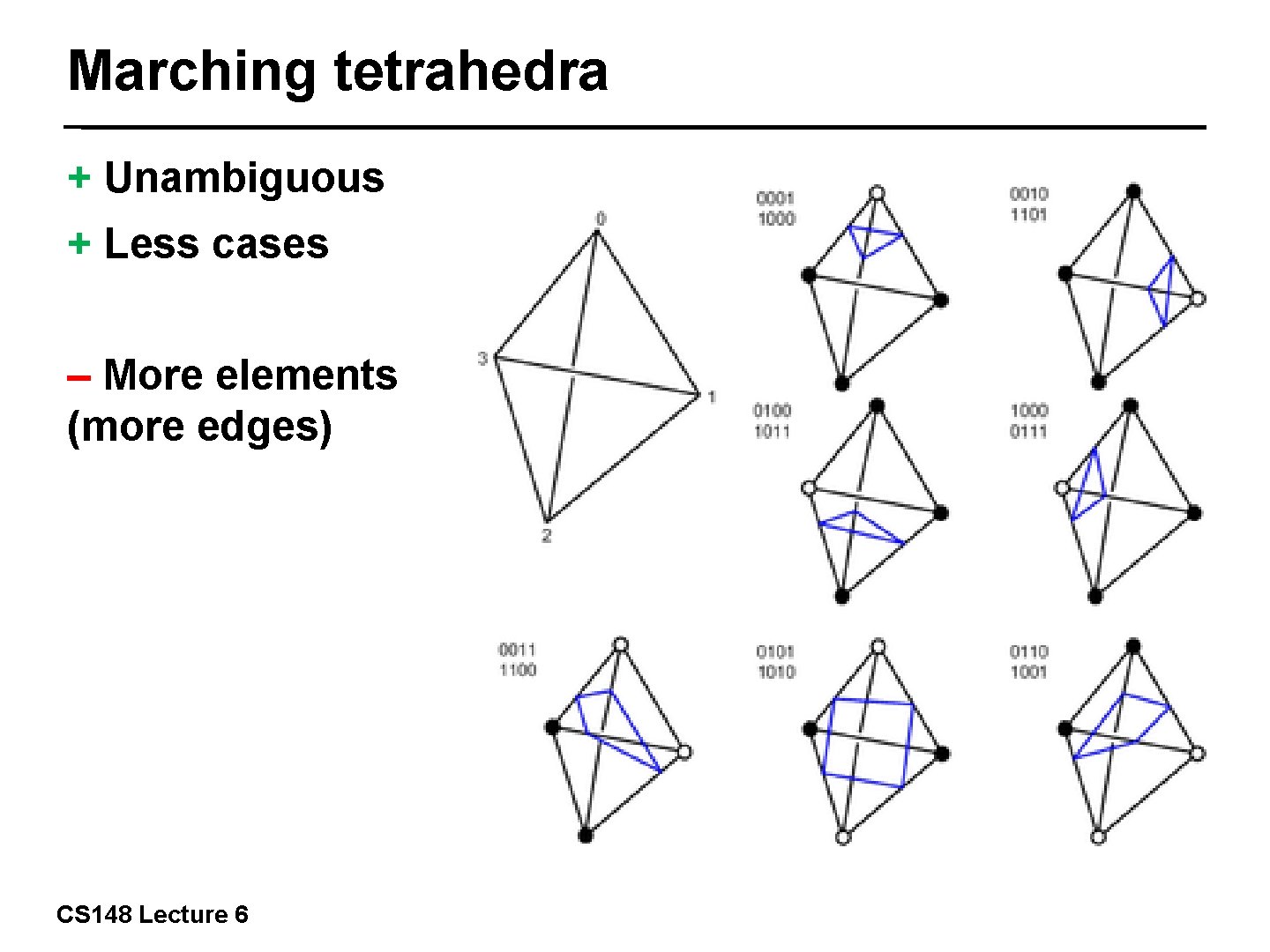
Marching tetrahedra + Unambiguous + Less cases – More elements (more edges) 45/57 CS 148 Lecture 6

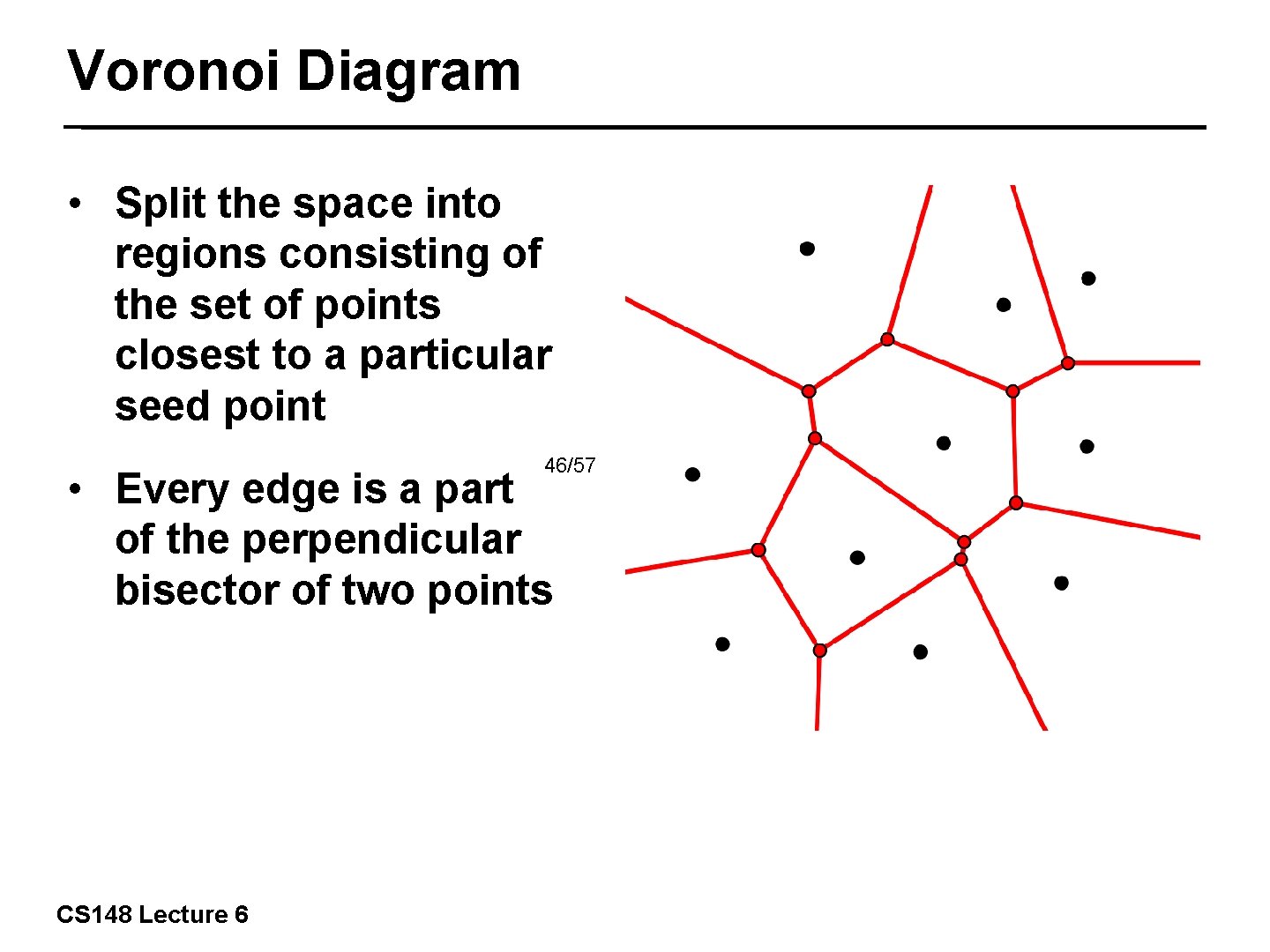
Voronoi Diagram • Split the space into regions consisting of the set of points closest to a particular seed point 46/57 • Every edge is a part of the perpendicular bisector of two points CS 148 Lecture 6

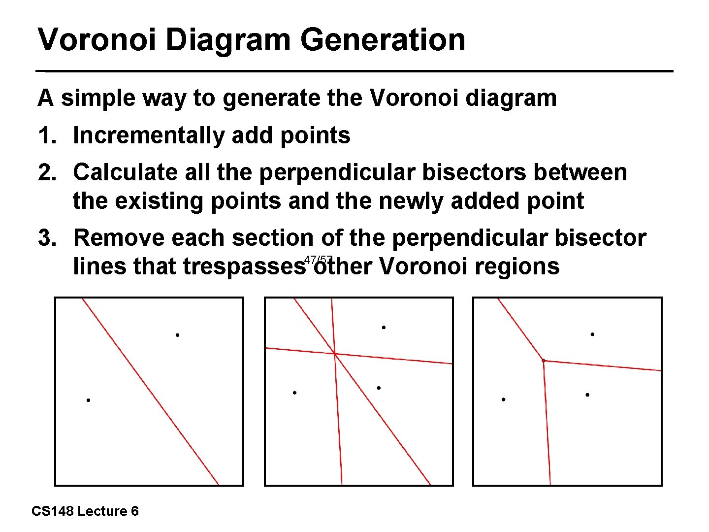
Voronoi Diagram Generation A simple way to generate the Voronoi diagram 1. Incrementally add points 2. Calculate all the perpendicular bisectors between the existing points and the newly added point 3. Remove each section of the perpendicular bisector 47/57 lines that trespasses other Voronoi regions CS 148 Lecture 6

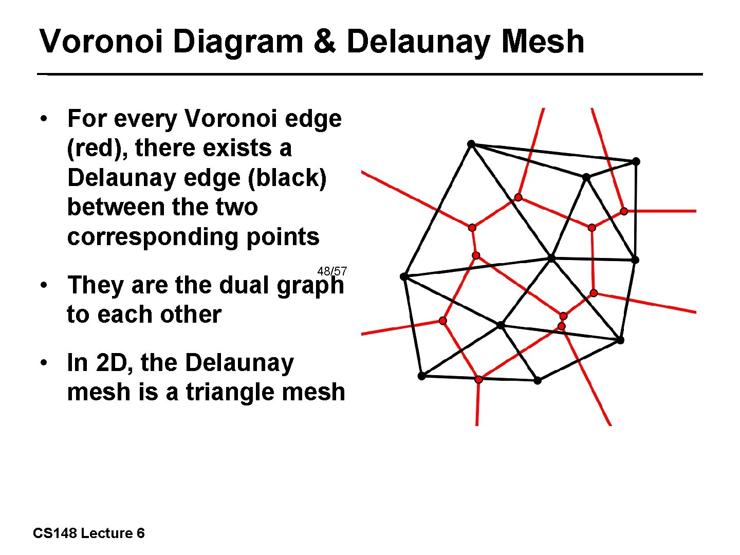
Voronoi Diagram & Delaunay Mesh • For every Voronoi edge (red), there exists a Delaunay edge (black) between the two corresponding points 48/57 • They are the dual graph to each other • In 2 D, the Delaunay mesh is a triangle mesh CS 148 Lecture 6

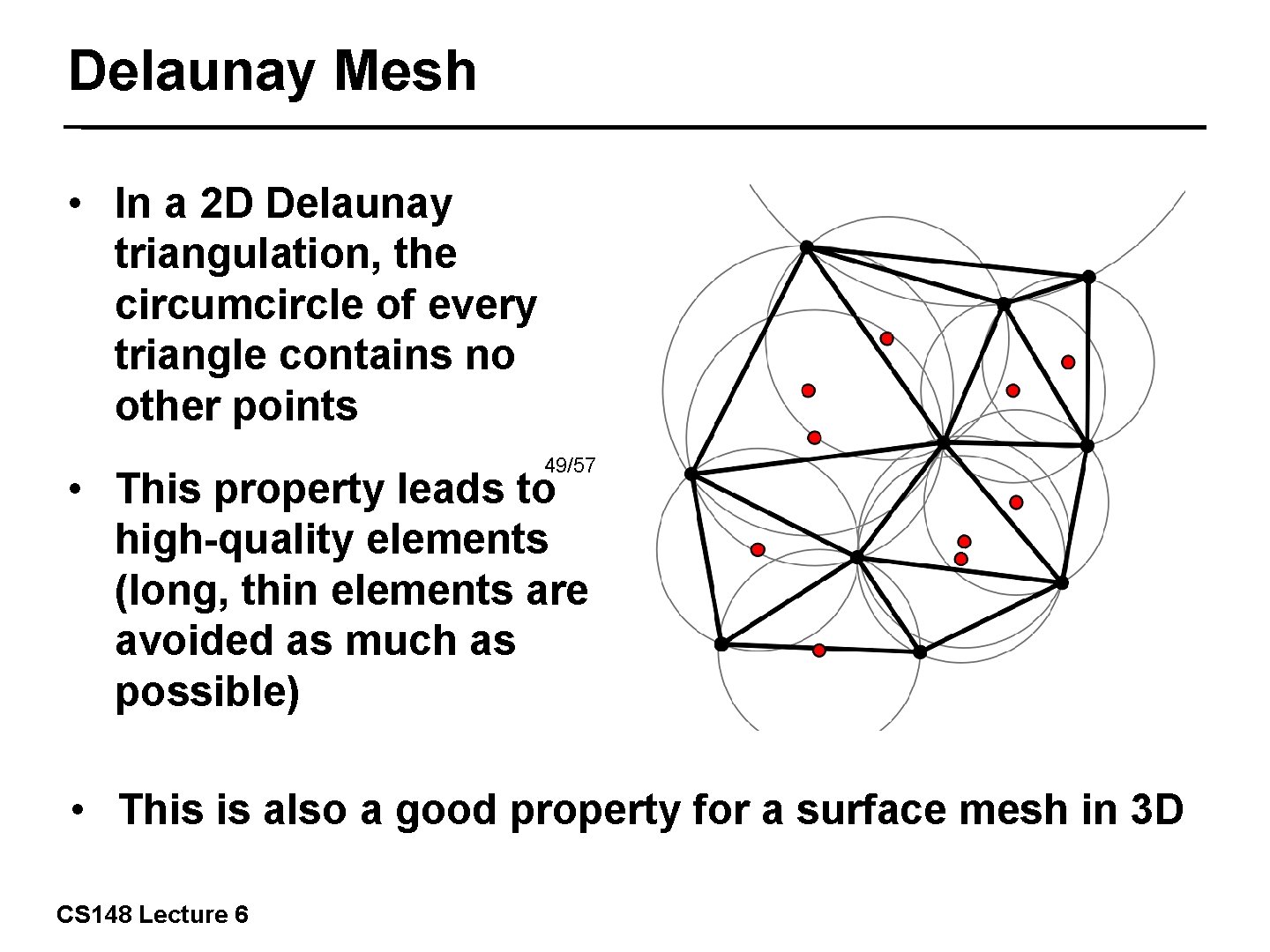
Delaunay Mesh • In a 2 D Delaunay triangulation, the circumcircle of every triangle contains no other points 49/57 • This property leads to high-quality elements (long, thin elements are avoided as much as possible) • This is also a good property for a surface mesh in 3 D CS 148 Lecture 6

Improving and Existing Mesh Edge-Flipping • In-Circle Test - for a pair of adjacent triangles, test whether the circumcircle of one triangle contains the fourth point • Flip the edge to make it locally-Delaunay 50/57 CS 148 Lecture 6

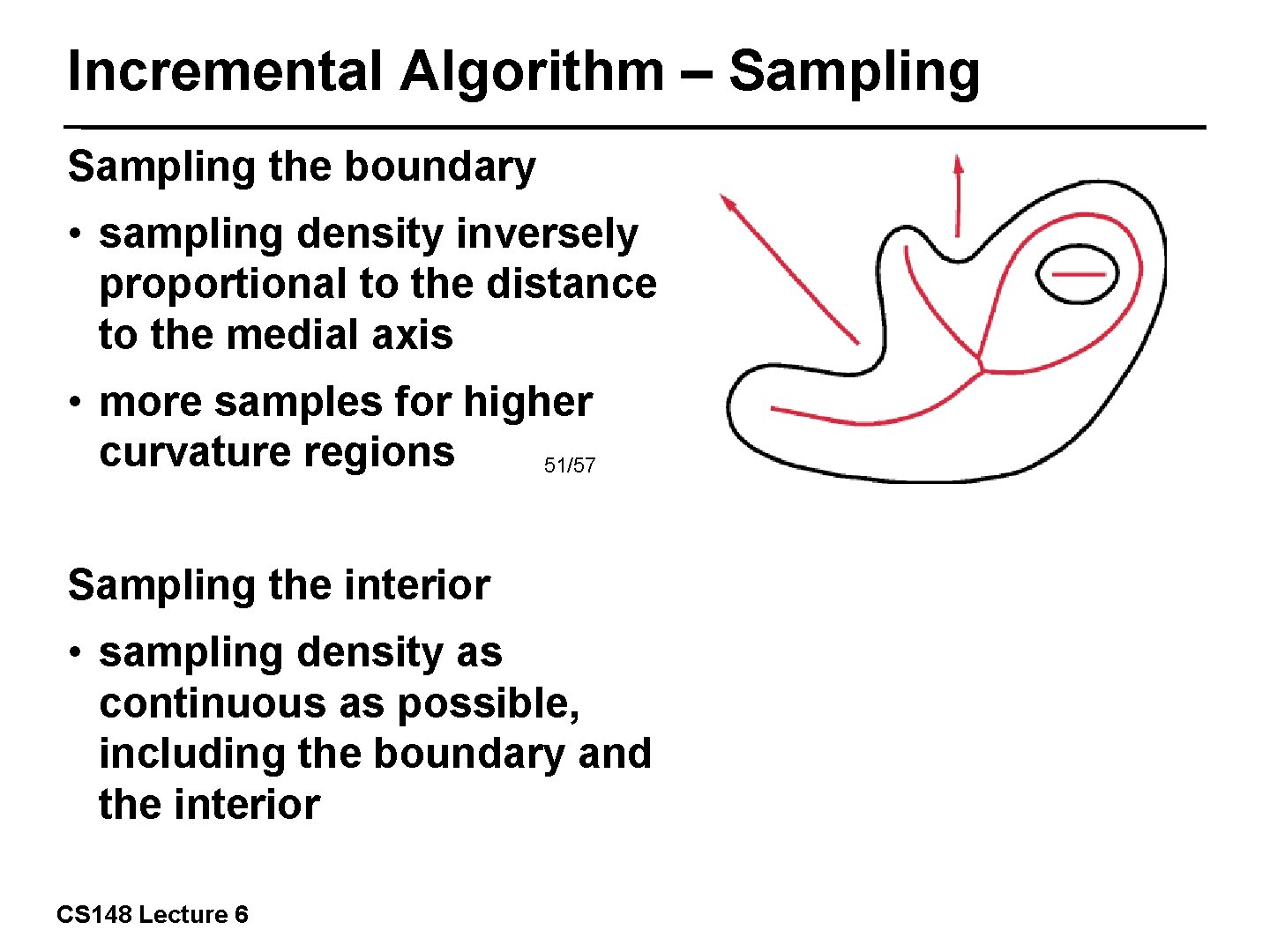
Incremental Algorithm – Sampling the boundary • sampling density inversely proportional to the distance to the medial axis • more samples for higher curvature regions 51/57 Sampling the interior • sampling density as continuous as possible, including the boundary and the interior CS 148 Lecture 6

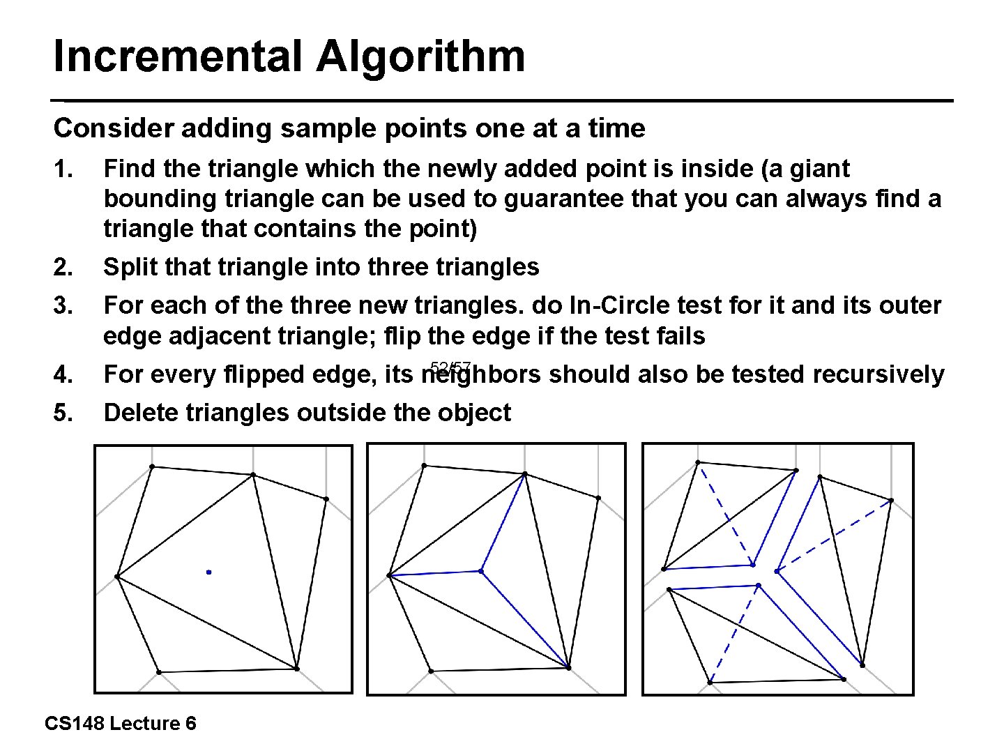
Incremental Algorithm Consider adding sample points one at a time 1. Find the triangle which the newly added point is inside (a giant bounding triangle can be used to guarantee that you can always find a triangle that contains the point) 2. Split that triangle into three triangles 3. For each of the three new triangles. do In-Circle test for it and its outer edge adjacent triangle; flip the edge if the test fails 52/57 4. For every flipped edge, its neighbors should also be tested recursively 5. Delete triangles outside the object CS 148 Lecture 6

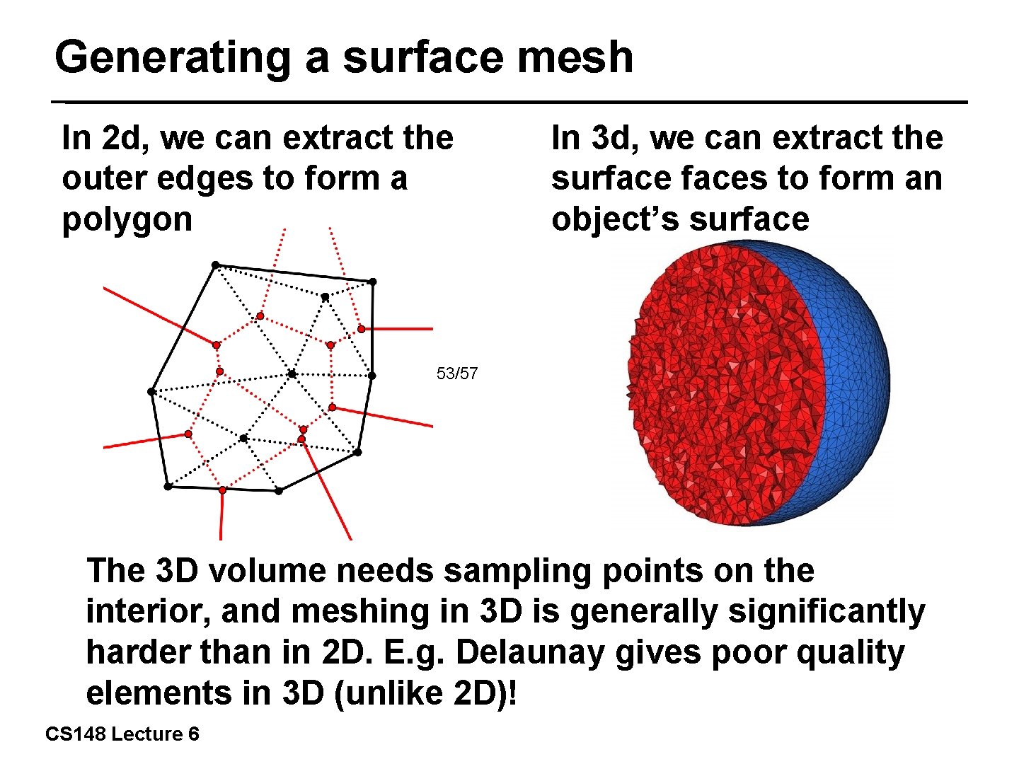
Generating a surface mesh In 2 d, we can extract the outer edges to form a polygon In 3 d, we can extract the surfaces to form an object’s surface 53/57 The 3 D volume needs sampling points on the interior, and meshing in 3 D is generally significantly harder than in 2 D. E. g. Delaunay gives poor quality elements in 3 D (unlike 2 D)! CS 148 Lecture 6

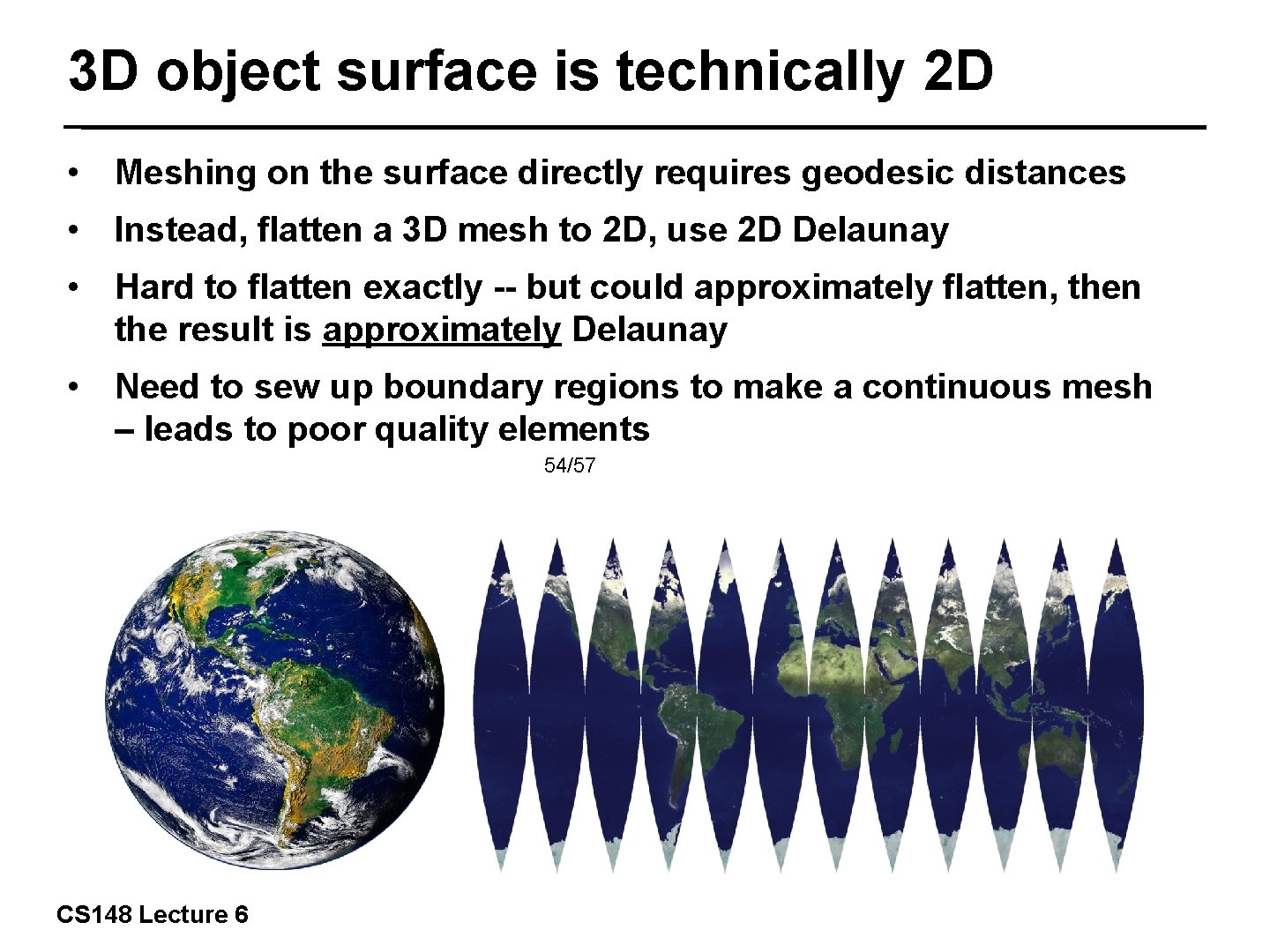
3 D object surface is technically 2 D • Meshing on the surface directly requires geodesic distances • Instead, flatten a 3 D mesh to 2 D, use 2 D Delaunay • Hard to flatten exactly -- but could approximately flatten, then the result is approximately Delaunay • Need to sew up boundary regions to make a continuous mesh – leads to poor quality elements 54/57 CS 148 Lecture 6

3 D object surface is technically 2 D • Cut the object to flatten it, and add new sample points (blue) along the cut • Generate the Delaunay with incremental algorithm connecting both original 55/57 (black) and new (blue) sampling points • sew up the boundary edges (reconnect blue points) • Retest/remesh to improve the mesh, especially near the boundary edges CS 148 Lecture 6

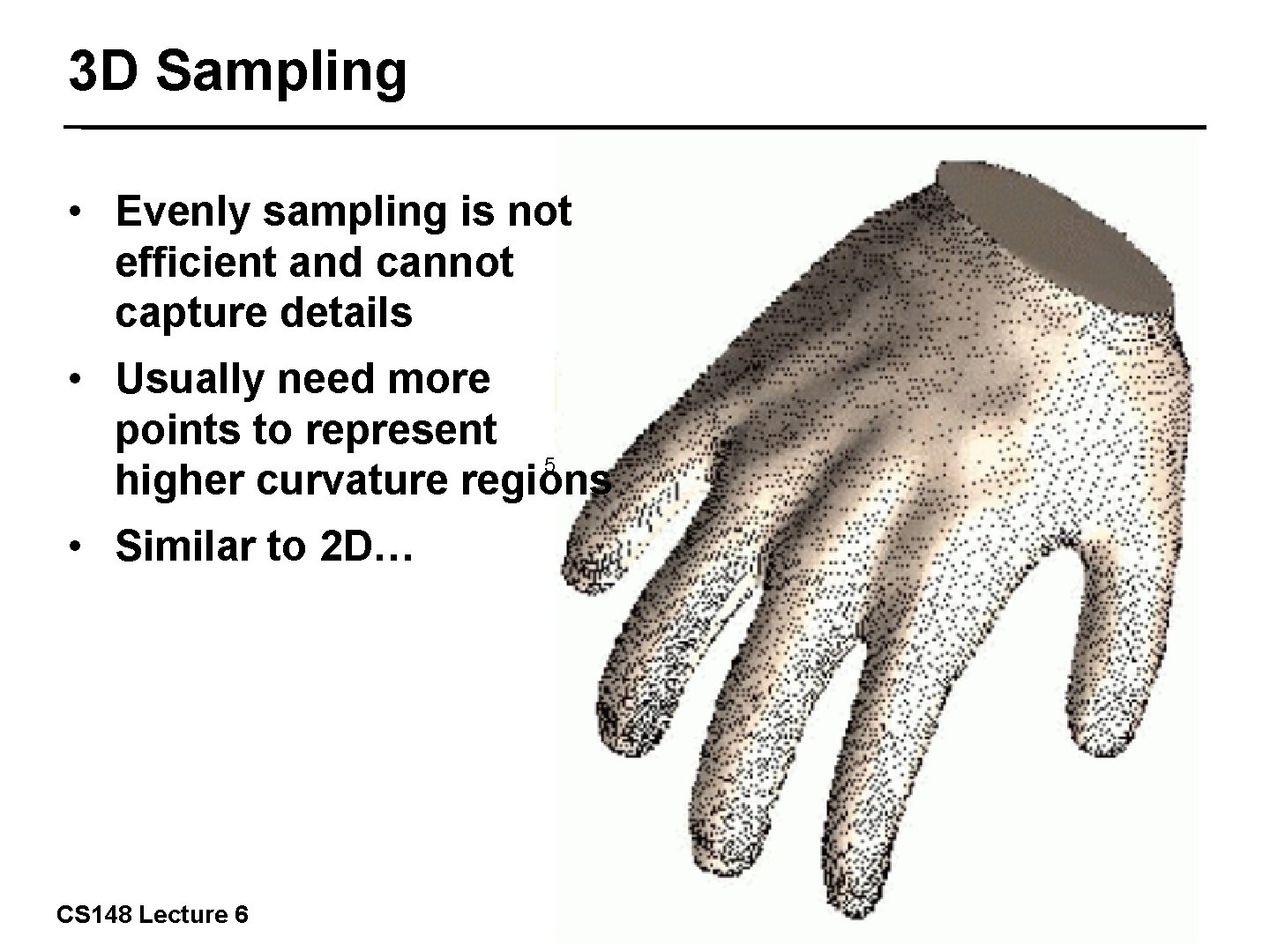
3 D Sampling • Evenly sampling is not efficient and cannot capture details • Usually need more points to represent 56/57 higher curvature regions • Similar to 2 D… CS 148 Lecture 6

3 D In-Circle Test • Once we get a 3 D mesh, the In-Circle test can be used to improve it, especially near the boundaries where it was sewn together • Need 3 D version of the In-Circle test • Use an ellipse to approximate the mapped circle in 57/57 2 D plane • Given three vertices on a curved surface, consider the infinite set of spheres through the three vertices. The centers of all the spheres lie on a single line. Choose the sphere whose center is on the surface and define In-Circle test as inside that sphere. CS 148 Lecture 6