CS 1321 CS 1321 Introduction to Programming Georgia

CS 1321

CS 1321: Introduction to Programming Georgia Institute of Technology College of Computing Lecture 24 November 15, 2001 Fall Semester

Today’s Menu 1. More Vectors 2. Complexity – How efficient is our plan of attack?

More Vectors & Loops Last time - concept of vectors. • like lists, store series of info sequentially. • unlike lists, • size of vector is statically bound and doesn’t change. (This fact allows us to know exactly where every item in the vector is in memory. Each can be accessed without traversing through all the items that exist prior to that item in our vector. Gain: direct access!) • vectors are not recursively defined data structures, so often vectors are processed using loops rather than recursion.

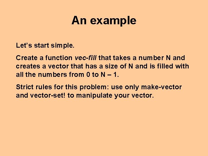
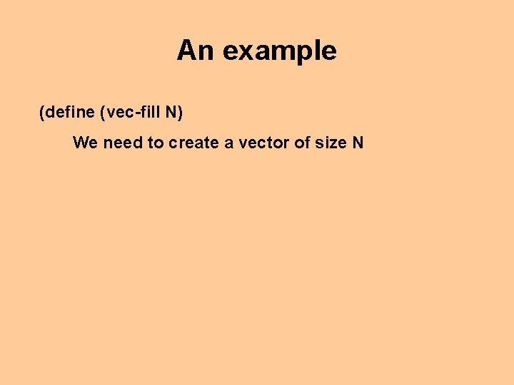
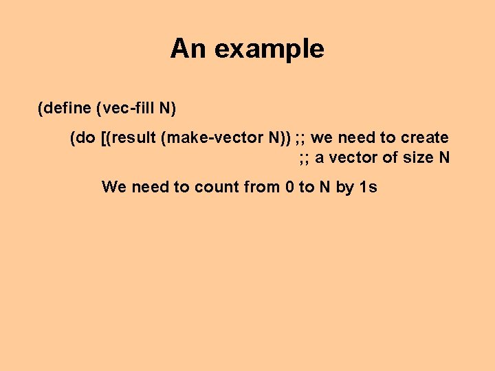
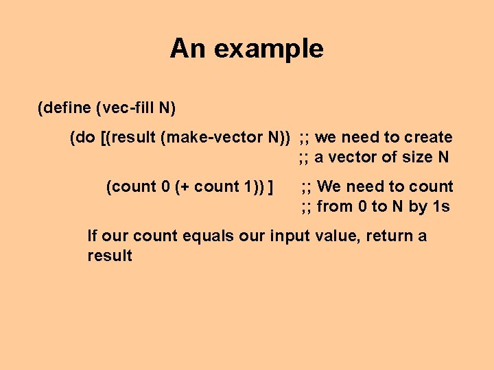
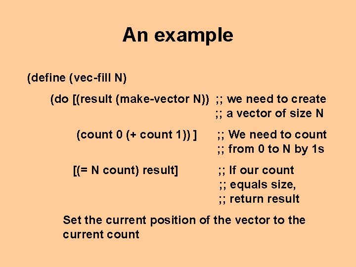
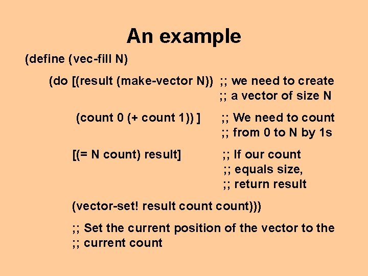
An example Let’s start simple. Create a function vec-fill that takes a number N and creates a vector that has a size of N and is filled with all the numbers from 0 to N – 1. Strict rules for this problem: use only make-vector and vector-set! to manipulate your vector.

An example (define (vec-fill N) We need to create a vector of size N

An example (define (vec-fill N) (do [(result (make-vector N)) ; ; we need to create ; ; a vector of size N We need to count from 0 to N by 1 s

An example (define (vec-fill N) (do [(result (make-vector N)) ; ; we need to create ; ; a vector of size N (count 0 (+ count 1)) ] ; ; We need to count ; ; from 0 to N by 1 s If our count equals our input value, return a result

An example (define (vec-fill N) (do [(result (make-vector N)) ; ; we need to create ; ; a vector of size N (count 0 (+ count 1)) ] [(= N count) result] ; ; We need to count ; ; from 0 to N by 1 s ; ; If our count ; ; equals size, ; ; return result Set the current position of the vector to the current count

An example (define (vec-fill N) (do [(result (make-vector N)) ; ; we need to create ; ; a vector of size N (count 0 (+ count 1)) ] [(= N count) result] ; ; We need to count ; ; from 0 to N by 1 s ; ; If our count ; ; equals size, ; ; return result (vector-set! result count))) ; ; Set the current position of the vector to the ; ; current count

The Matrix

You Must Choose Warning: The Slides Ahead are a challenge to your current concept of programming.

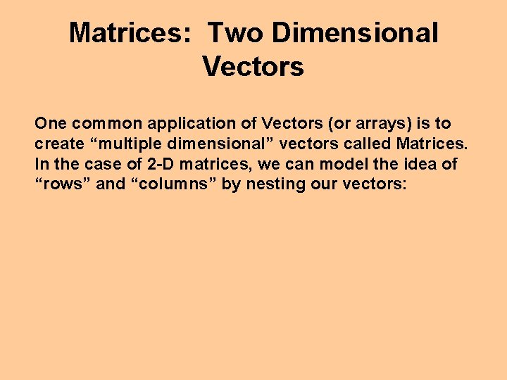
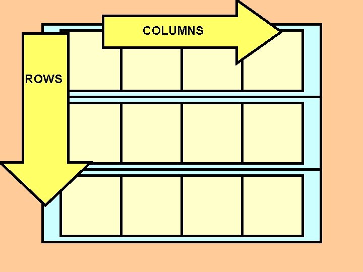
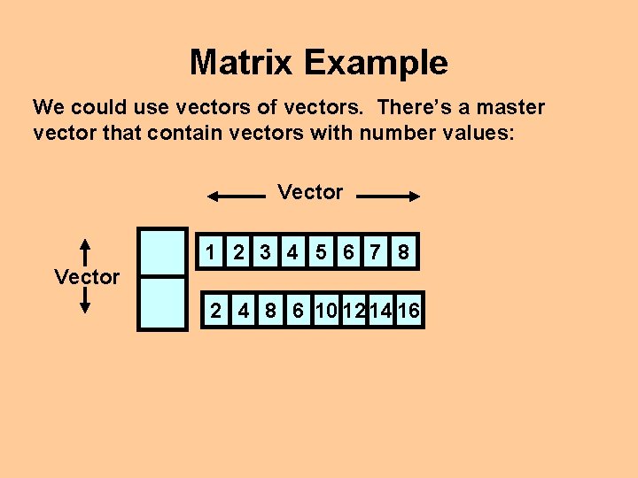
Matrices: Two Dimensional Vectors One common application of Vectors (or arrays) is to create “multiple dimensional” vectors called Matrices. In the case of 2 -D matrices, we can model the idea of “rows” and “columns” by nesting our vectors:

COLUMNS ROWS

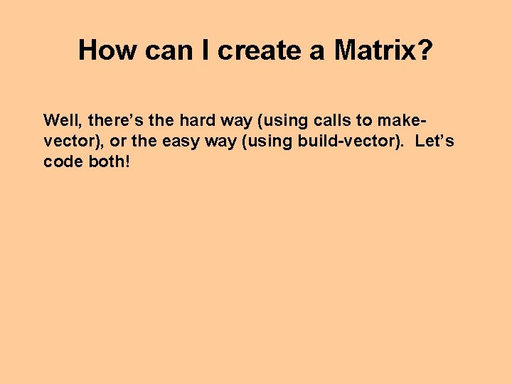
How can I create a Matrix? Well, there’s the hard way (using calls to makevector), or the easy way (using build-vector). Let’s code both!

Making matrices with makevector (define (make-matrix row column) (let [(matrix (make-vector row))] (do [(count 0 (+ count 1))] [(= count row) matrix] (vector-set! matrix count (make-vector column)))))

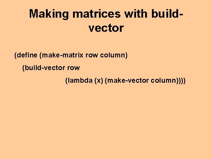
Making matrices with buildvector (define (make-matrix row column) (build-vector row (lambda (x) (make-vector column))))

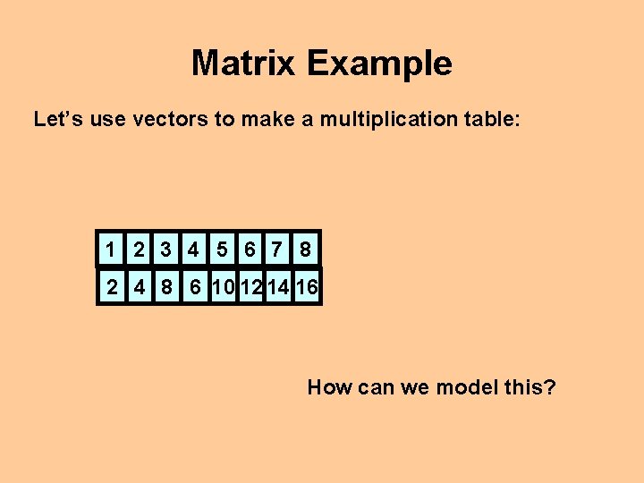
Hey kids, remember multiplication tables? Remember, we can use build-vector to seed each element of our vector with some initial value. That’s how we used it to create a matrix. Why don’t we alter our make-matrix example to start our matrix out with all the entries in an M x N multiplication table?

Matrix Example Let’s use vectors to make a multiplication table: 1 2 3 4 5 6 7 8 2 4 8 6 10 12 14 16 How can we model this?

Matrix Example We could use vectors of vectors. There’s a master vector that contain vectors with number values: Vector 1 2 3 4 5 6 7 8 Vector 2 4 8 6 10 12 14 16

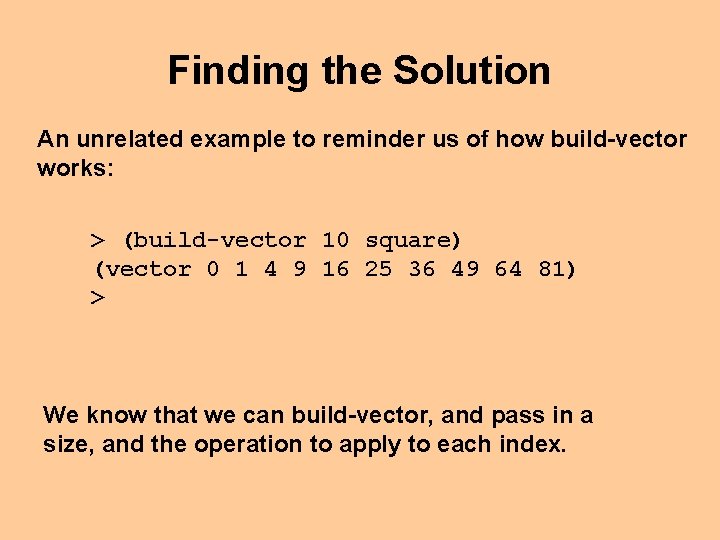
Finding the Solution An unrelated example to reminder us of how build-vector works: > (build-vector 10 square) (vector 0 1 4 9 16 25 36 49 64 81) > We know that we can build-vector, and pass in a size, and the operation to apply to each index.

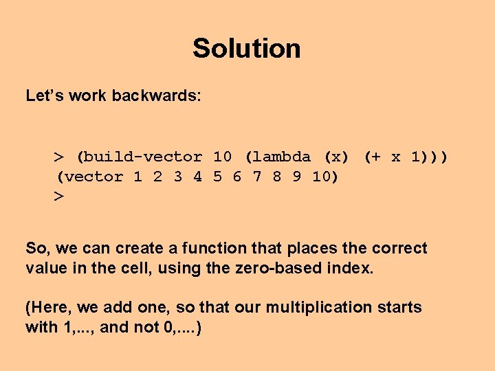
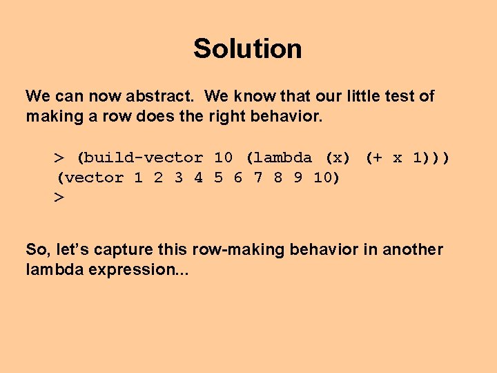
Solution Let’s work backwards: > (build-vector 10 (lambda (x) (+ x 1))) (vector 1 2 3 4 5 6 7 8 9 10) > So, we can create a function that places the correct value in the cell, using the zero-based index. (Here, we add one, so that our multiplication starts with 1, . . . , and not 0, . . )

Solution We can now abstract. We know that our little test of making a row does the right behavior. > (build-vector 10 (lambda (x) (+ x 1))) (vector 1 2 3 4 5 6 7 8 9 10) > So, let’s capture this row-making behavior in another lambda expression. . .

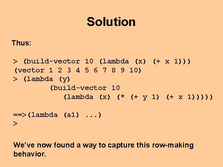
Solution Thus: > (build-vector 10 (lambda (x) (+ x 1))) (vector 1 2 3 4 5 6 7 8 9 10) > (lambda (y) (build-vector 10 (lambda (x) (* (+ y 1) (+ x 1))))) ==>(lambda (a 1). . . ) > We’ve now found a way to capture this row-making behavior.

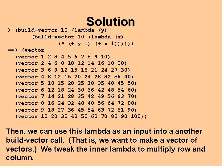
Solution > (build-vector 10 (lambda (y) (build-vector 10 (lambda (x) (* (+ y 1) (+ x 1)))))) ==> (vector 1 2 3 4 5 6 7 8 9 10) (vector 2 4 6 8 10 12 14 16 18 20) (vector 3 6 9 12 15 18 21 24 27 30) (vector 4 8 12 16 20 24 28 32 36 40) (vector 5 10 15 20 25 30 35 40 45 50) (vector 6 12 18 24 30 36 42 48 54 60) (vector 7 14 21 28 35 42 49 56 63 70) (vector 8 16 24 32 40 48 56 64 72 80) (vector 9 18 27 36 45 54 63 72 81 90) (vector 10 20 30 40 50 60 70 80 90 100)) Then, we can use this lambda as an input into a another build-vector call. (That is, we want to make a vector of vectors. ) We tweak the inner lambda to multiply row and column.

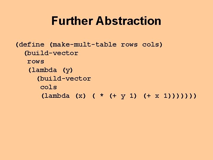
Further Abstraction (define (make-mult-table rows cols) (build-vector rows (lambda (y) (build-vector cols (lambda (x) ( * (+ y 1) (+ x 1)))))))

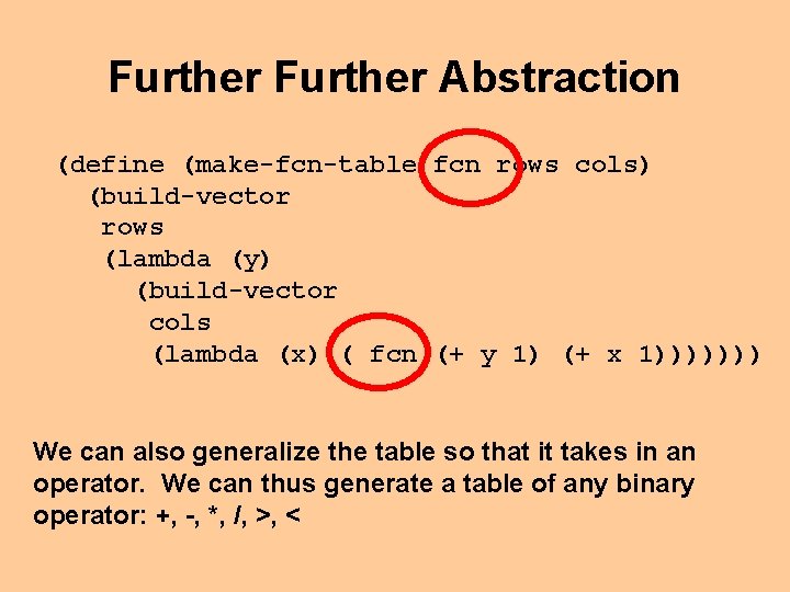
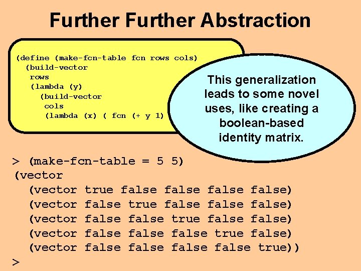
Further Abstraction (define (make-fcn-table fcn rows cols) (build-vector rows (lambda (y) (build-vector cols (lambda (x) ( fcn (+ y 1) (+ x 1))))))) We can also generalize the table so that it takes in an operator. We can thus generate a table of any binary operator: +, -, *, /, >, <

Further Abstraction (define (make-fcn-table fcn rows cols) (build-vector rows This generalization (lambda (y) leads to some novel (build-vector cols uses, like creating a (lambda (x) ( fcn (+ y 1) (+ x 1))))))) boolean-based identity matrix. > (make-fcn-table = 5 5) (vector true false false) (vector false true false) (vector false false true)) >

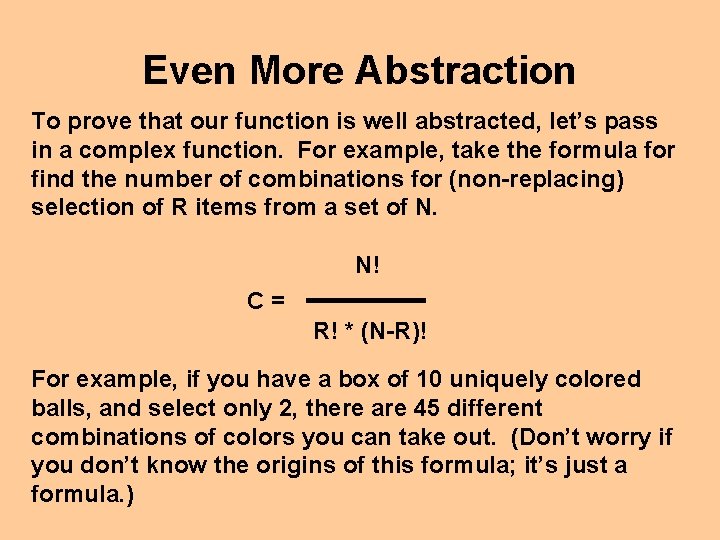
Even More Abstraction To prove that our function is well abstracted, let’s pass in a complex function. For example, take the formula for find the number of combinations for (non-replacing) selection of R items from a set of N. N! C= R! * (N-R)! For example, if you have a box of 10 uniquely colored balls, and select only 2, there are 45 different combinations of colors you can take out. (Don’t worry if you don’t know the origins of this formula; it’s just a formula. )

Further Abstraction (define (factorial n) (cond This should look [ (zero? n) 1 ] familiar. . . [ else (* n (factorial (- n 1)))])) This is just a Scheme version of the formula, with a little safety checking. (The number of selections can’t exceed the number of items to choose from. ) (define (combinations n r) (cond [ (> r n) 'none ] [ else (/ (factorial n) (* (factorial r) (factorial (- n r))))]))

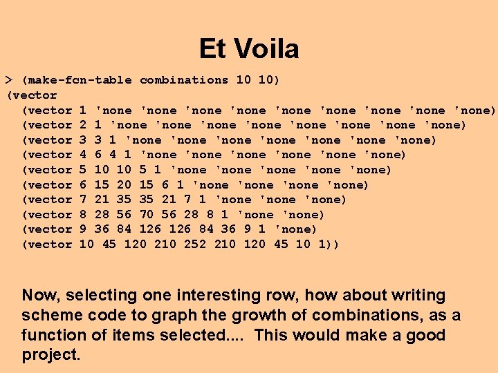
Et Voila > (make-fcn-table combinations 10 10) (vector 1 'none 'none 'none) (vector 2 1 'none 'none) (vector 3 3 1 'none 'none) (vector 4 6 4 1 'none 'none) (vector 5 10 10 5 1 'none 'none) (vector 6 15 20 15 6 1 'none) (vector 7 21 35 35 21 7 1 'none) (vector 8 28 56 70 56 28 8 1 'none) (vector 9 36 84 126 84 36 9 1 'none) (vector 10 45 120 210 252 210 120 45 10 1)) Now, selecting one interesting row, how about writing scheme code to graph the growth of combinations, as a function of items selected. . This would make a good project.

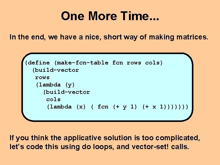
One More Time. . . In the end, we have a nice, short way of making matrices. (define (make-fcn-table fcn rows cols) (build-vector rows (lambda (y) (build-vector cols (lambda (x) ( fcn (+ y 1) (+ x 1))))))) If you think the applicative solution is too complicated, let’s code this using do loops, and vector-set! calls.

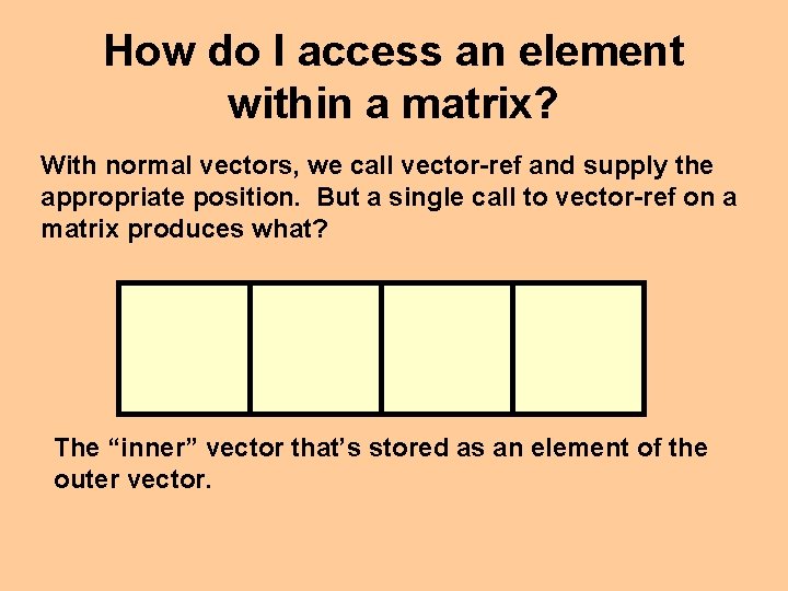
How do I access an element within a matrix? With normal vectors, we call vector-ref and supply the appropriate position. But a single call to vector-ref on a matrix produces what? The “inner” vector that’s stored as an element of the outer vector.

So working with matrices takes a bit more effort. Let’s work from an example. Let’s say we wanted to duplicate the efforts of our multiplication table the hard way: by going through each element of the matrix one at a time and calculating the appropriate multiplication at that point. Let’s make it more interesting by taking in a matrix of unknown size as well…

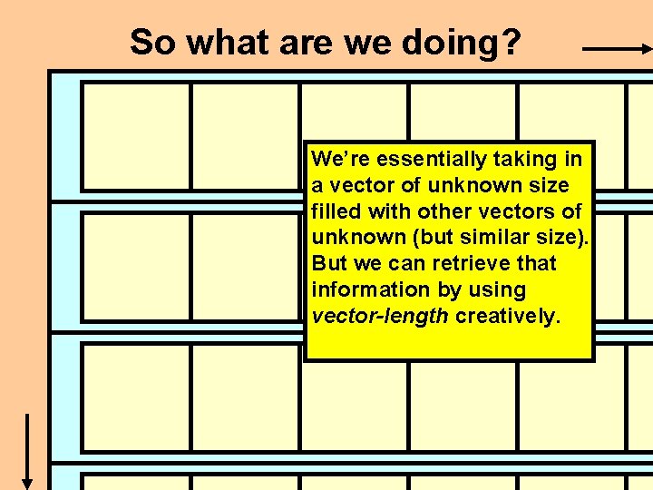
So what are we doing? We’re essentially taking in a vector of unknown size filled with other vectors of unknown (but similar size). But we can retrieve that information by using vector-length creatively.

(define (make-mult in-matrix) (let [(row (vector-length in-matrix)) (col (vector-length (vector-ref in-matrix 0)))] What does this mean?

So now we have this notion of the total number of rows, and the total number of columns in our matrix. Let’s start by handling one row at a time…

(define (make-mult in-matrix) (let [(row (vector-length in-matrix)) (col (vector-length (vector-ref in-matrix 0)))] (do [(row-count 0 (+ count 1))] [(= row-count row) in-matrix] …(vector-ref in-matrix row-count) … )))

Inside each of those rows, we want to travel to each of our column entries and store our calculated value of the current row by the current column.

(define (make-mult in-matrix) (let [(row (vector-length in-matrix)) (col (vector-length (vector-ref in-matrix 0)))] (do [(row-count 0 (+ row-count 1))] [(= row-count row) in-matrix] (do [(col-count 0 (+ col-count 1))] [(= col-count col) in-matrix] (vector-set! (vector-ref in-matrix row-count) col-count ( * col-count row-count)) )))

(define (make-mult in-matrix) (let [(row (vector-length in-matrix)) (col (vector-length (vector-ref in-matrix 0)))] (do [(row-count 0 (+ row-count 1))] [(= row-count row)ugly in-matrix] Ouch! That’s some code! It’s a good thing we have applicative programming! (do [(col-count 0 (+ col-count 1))] [(= col-count col) in-matrix] But if we had to take this route, we might (vector-set! in-matrix want to think up some(vector-ref abstractions for some common matrix operations…. row-count) col-count ( * col-count row-count)) )))

“Just how good is my algorithm? ” How many times this semester have you asked yourself this question? Probably not very often, if ever. After all, we’ve been creating relatively simple programs that work on a small finite set of data. Our functions execute and return an answer with a second or two. So why worry?

“Just how good is my algorithm? ” In the real programming world, we usually work with much larger data sets • inventory of Wal-Mart™ • number of transactions handled by Wachovia™ on a day Then it becomes vitally important that we consider the relative “goodness” of the algorithm we’re considering. In other words, as the amount of data increases, we must care how much our implementation costs us in terms of time, memory & effort!

Big O is a mathematical concept that attempts to express just how “good” or “bad” a particular thought process or algorithm is. Please note that the concept as we explain it in CS 1321 is a greatly simplified version of explaining the complexity of an algorithm. In later courses, you’ll be introduced to a more formal definition of Big-O, along with its various relatives: little-O, Big- , little- , and Big-.

The Story of Big O, as noted in this class, is a measure of the “worst-case” scenario for a given algorithm taking in input of size N. Mathematically: Given an input of size N (where N is really big), what is the asymptotic upper bounds of the algorithm in terms of time/space (how long will it take to execute/how much memory will it require)?

O(? ) There a few common notations for Big-O. These are categories into which almost all algorithms fit into (once we through away all the garbage and reduce the algorithm to its purest form). These are denoted as follows: • O(1) • O(N M) • O(log N) • O(M N) • O(N) • Or some combination of these.

O(1): What Computer Scientists Dream About O(1) doesn’t mean we finish everything in one second or one CPU cycle or that our algorithm only uses one layer of the stack rather than building and building. We just wish that it did. O(1) means constant time or space. No matter what we through at a particular algorithm, we know EXACTLY how long/how much it will take to execute the program: Given a vector of size N (where N is unknown), access a particular value. Given a list of size P (where P is unknown), retrieve the first element of the list.

O(N): Searching Everywhere… This one’s pretty easy to see. If we have a list containing N elements, and we are searching for a particular value that isn’t even contained in the list, how many elements do we have to search through? N elements! Or how about searching through a Binary Tree (not a BST) of size N for a value that doesn’t exist? O(N).

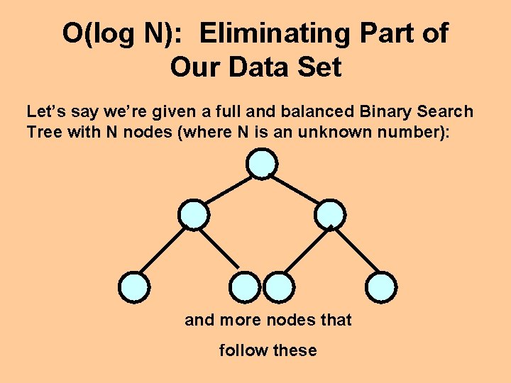
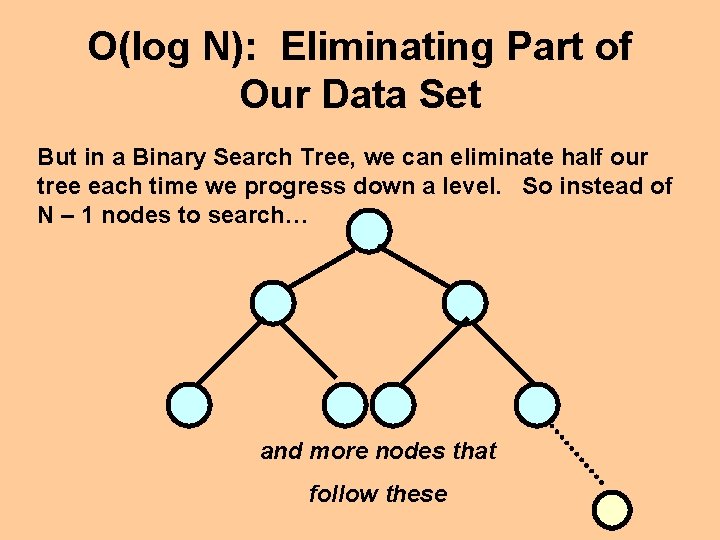
O(log N): Eliminating Part of Our Data Set Let’s say we’re given a full and balanced Binary Search Tree with N nodes (where N is an unknown number): and more nodes that follow these

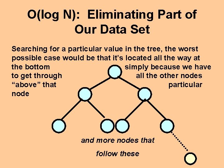
O(log N): Eliminating Part of Our Data Set Searching for a particular value in the tree, the worst possible case would be that it’s located all the way at the bottom simply because we have to get through all the other nodes “above” that particular node and more nodes that follow these

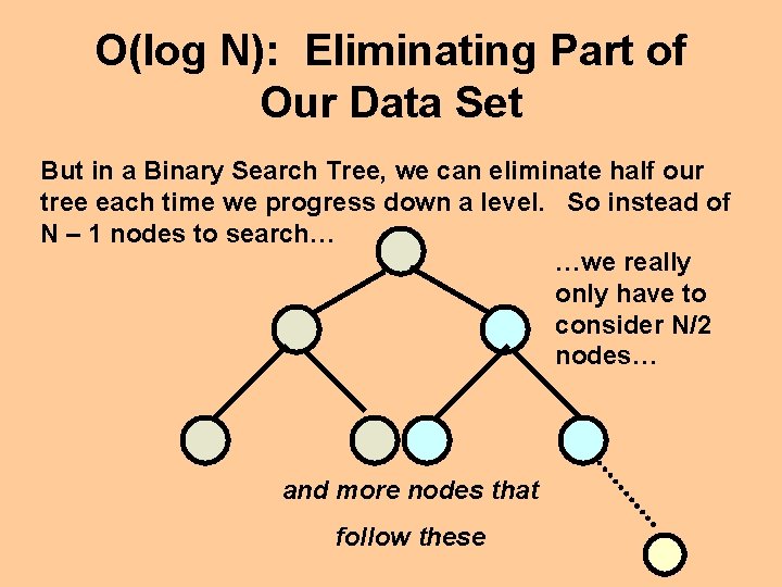
O(log N): Eliminating Part of Our Data Set But in a Binary Search Tree, we can eliminate half our tree each time we progress down a level. So instead of N – 1 nodes to search… and more nodes that follow these

O(log N): Eliminating Part of Our Data Set But in a Binary Search Tree, we can eliminate half our tree each time we progress down a level. So instead of N – 1 nodes to search… …we really only have to consider N/2 nodes… and more nodes that follow these

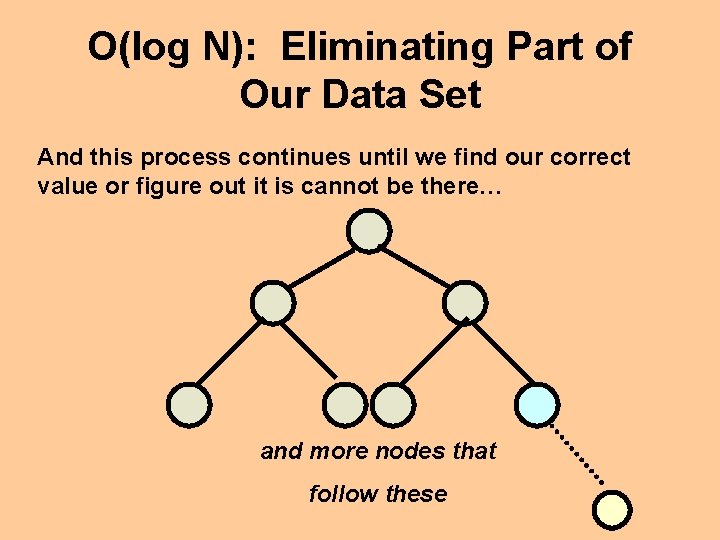
O(log N): Eliminating Part of Our Data Set And this process continues until we find our correct value or figure out it is cannot be there… and more nodes that follow these

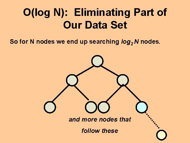
O(log N): Eliminating Part of Our Data Set So for N nodes we end up searching log 2 N nodes. and more nodes that follow these

O(log N): Eliminating Part of Our Data Set This holds true for any particular algorithm that eliminates a large portion of the data set each time it repeats. It’s generalized into O(log N).

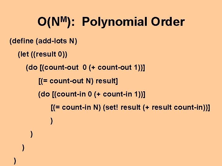
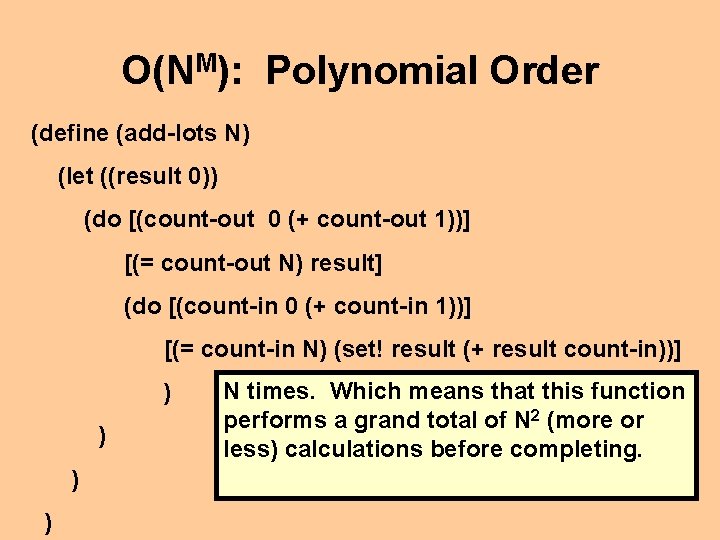
O(NM): Polynomial Order (define (add-lots N) (let ((result 0)) (do [(count-out 0 (+ count-out 1))] [(= count-out N) result] (do [(count-in 0 (+ count-in 1))] [(= count-in N) (set! result (+ result count-in))] ) )

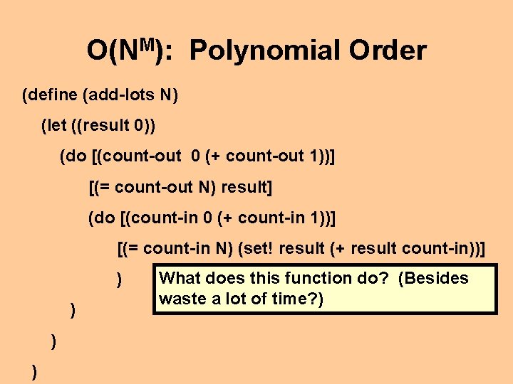
O(NM): Polynomial Order (define (add-lots N) (let ((result 0)) (do [(count-out 0 (+ count-out 1))] [(= count-out N) result] (do [(count-in 0 (+ count-in 1))] [(= count-in N) (set! result (+ result count-in))] ) ) What does this function do? (Besides waste a lot of time? )

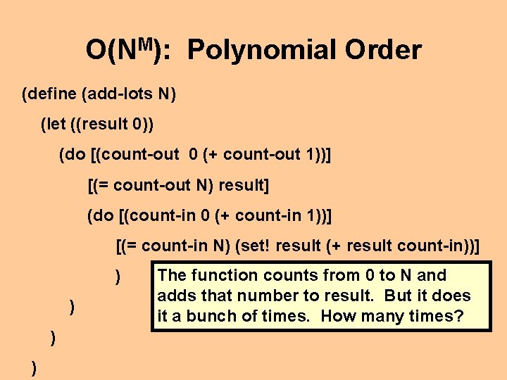
O(NM): Polynomial Order (define (add-lots N) (let ((result 0)) (do [(count-out 0 (+ count-out 1))] [(= count-out N) result] (do [(count-in 0 (+ count-in 1))] [(= count-in N) (set! result (+ result count-in))] ) ) The function counts from 0 to N and adds that number to result. But it does it a bunch of times. How many times?

O(NM): Polynomial Order (define (add-lots N) (let ((result 0)) (do [(count-out 0 (+ count-out 1))] [(= count-out N) result] (do [(count-in 0 (+ count-in 1))] [(= count-in N) (set! result (+ result count-in))] ) ) N times. Which means that this function performs a grand total of N 2 (more or less) calculations before completing.

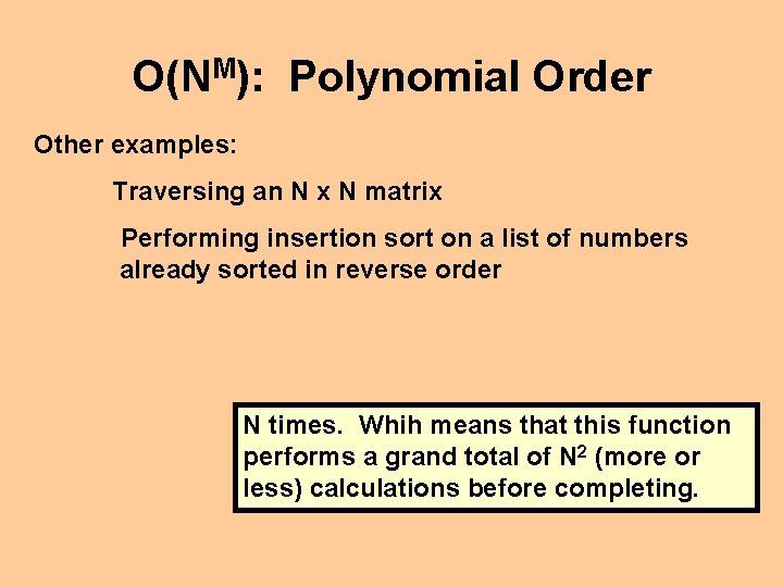
O(NM): Polynomial Order Other examples: Traversing an N x N matrix Performing insertion sort on a list of numbers already sorted in reverse order N times. Whih means that this function performs a grand total of N 2 (more or less) calculations before completing.

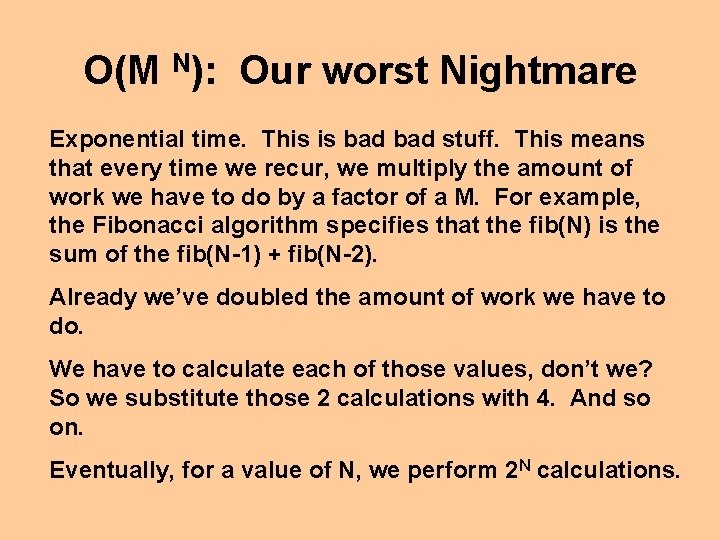
O(M N): Our worst Nightmare Exponential time. This is bad stuff. This means that every time we recur, we multiply the amount of work we have to do by a factor of a M. For example, the Fibonacci algorithm specifies that the fib(N) is the sum of the fib(N-1) + fib(N-2). Already we’ve doubled the amount of work we have to do. We have to calculate each of those values, don’t we? So we substitute those 2 calculations with 4. And so on. Eventually, for a value of N, we perform 2 N calculations.

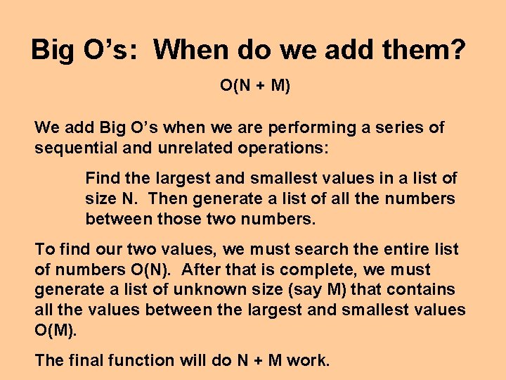
Big O’s: When do we add them? O(N + M) We add Big O’s when we are performing a series of sequential and unrelated operations: Find the largest and smallest values in a list of size N. Then generate a list of all the numbers between those two numbers. To find our two values, we must search the entire list of numbers O(N). After that is complete, we must generate a list of unknown size (say M) that contains all the values between the largest and smallest values O(M). The final function will do N + M work.

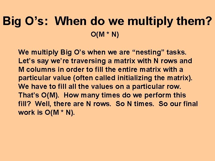
Big O’s: When do we multiply them? O(M * N) We multiply Big O’s when we are “nesting” tasks. Let’s say we’re traversing a matrix with N rows and M columns in order to fill the entire matrix with a particular value (often called initializing the matrix). We have to fill all the values on a particular row. That’s O(M). How many times do we perform this fill? Well, there are N rows. So N times. So our final work is O(M * N).

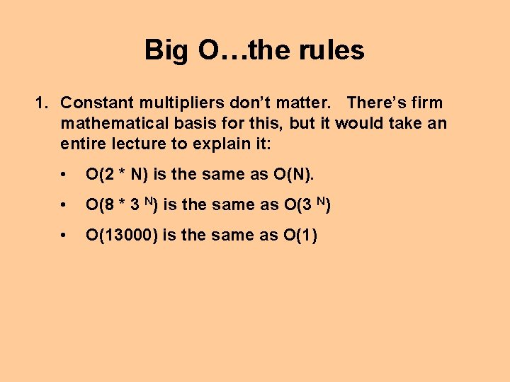
Big O…the rules 1. Constant multipliers don’t matter. There’s firm mathematical basis for this, but it would take an entire lecture to explain it: • O(2 * N) is the same as O(N). • O(8 * 3 N) is the same as O(3 N) • O(13000) is the same as O(1)

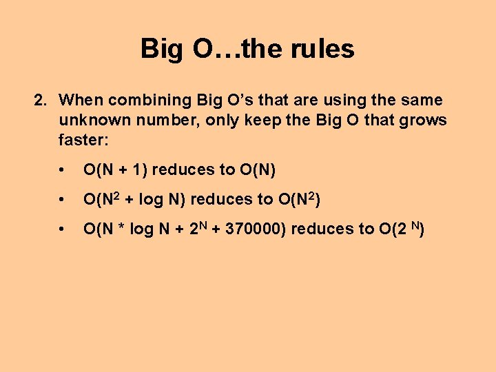
Big O…the rules 2. When combining Big O’s that are using the same unknown number, only keep the Big O that grows faster: • O(N + 1) reduces to O(N) • O(N 2 + log N) reduces to O(N 2) • O(N * log N + 2 N + 370000) reduces to O(2 N)

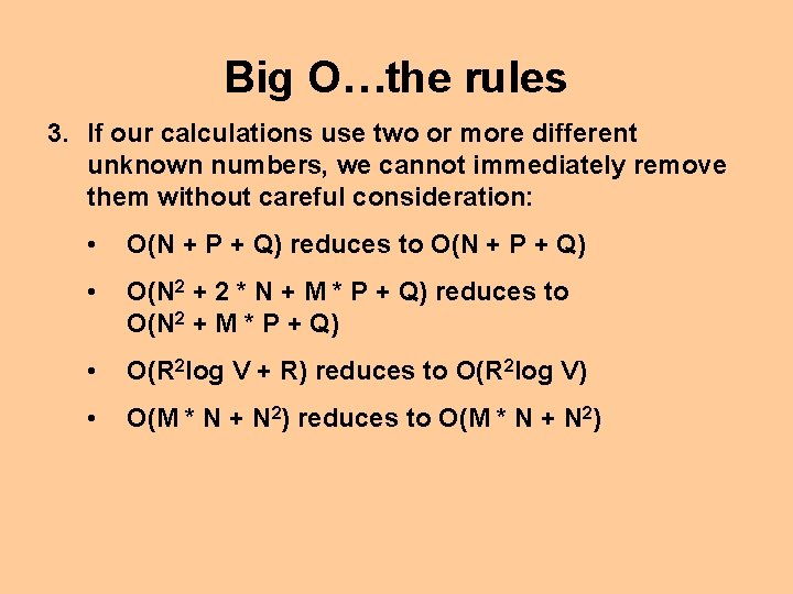
Big O…the rules 3. If our calculations use two or more different unknown numbers, we cannot immediately remove them without careful consideration: • O(N + P + Q) reduces to O(N + P + Q) • O(N 2 + 2 * N + M * P + Q) reduces to O(N 2 + M * P + Q) • O(R 2 log V + R) reduces to O(R 2 log V) • O(M * N + N 2) reduces to O(M * N + N 2)