Cracking the Code Using quantitative models in Matlab

Cracking the Code: Using quantitative models in Matlab to solve problems M. Letitia Hubbard, Ph. D North Carolina School of Science and Math, Durham, NC

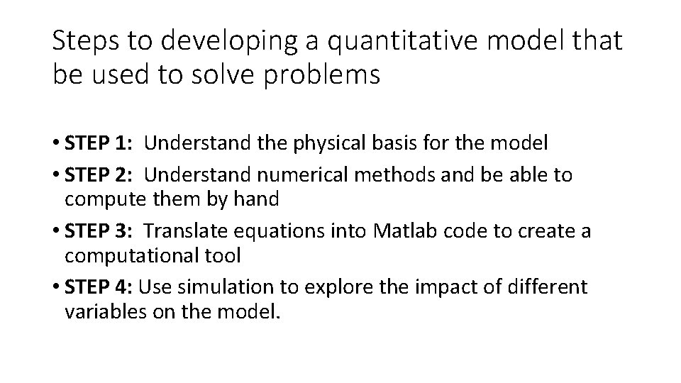
Steps to developing a quantitative model that be used to solve problems • STEP 1: Understand the physical basis for the model • STEP 2: Understand numerical methods and be able to compute them by hand • STEP 3: Translate equations into Matlab code to create a computational tool • STEP 4: Use simulation to explore the impact of different variables on the model.

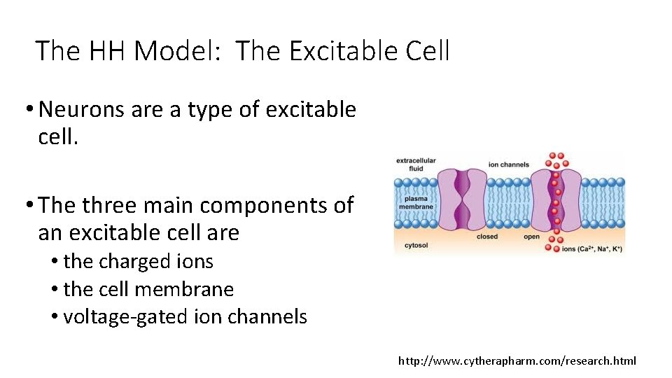
The HH Model: The Excitable Cell • Neurons are a type of excitable cell. • The three main components of an excitable cell are • the charged ions • the cell membrane • voltage-gated ion channels http: //www. cytherapharm. com/research. html

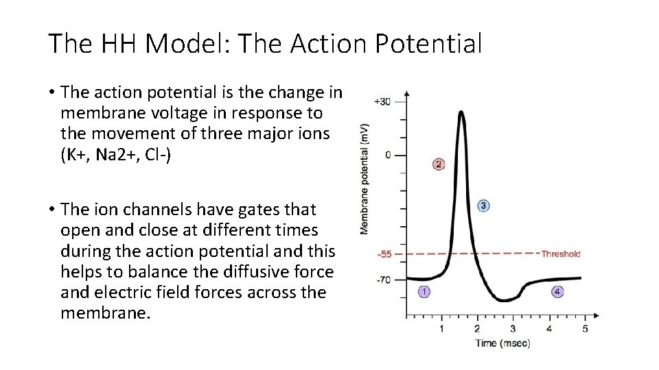
The HH Model: The Action Potential • The action potential is the change in membrane voltage in response to the movement of three major ions (K+, Na 2+, Cl-) • The ion channels have gates that open and close at different times during the action potential and this helps to balance the diffusive force and electric field forces across the membrane.

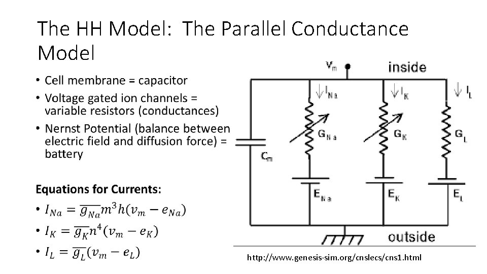
The HH Model: The Parallel Conductance Model • http: //www. genesis-sim. org/cnslecs/cns 1. html

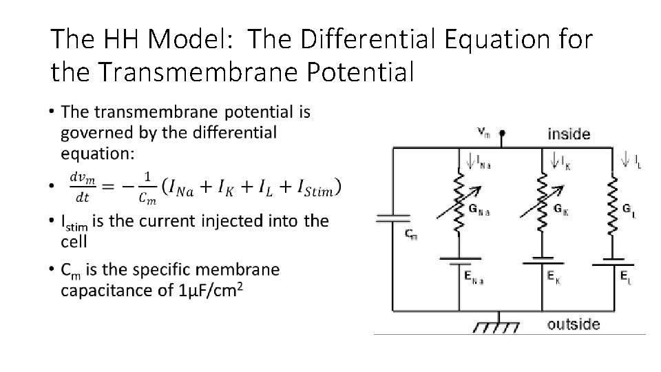
The HH Model: The Differential Equation for the Transmembrane Potential •

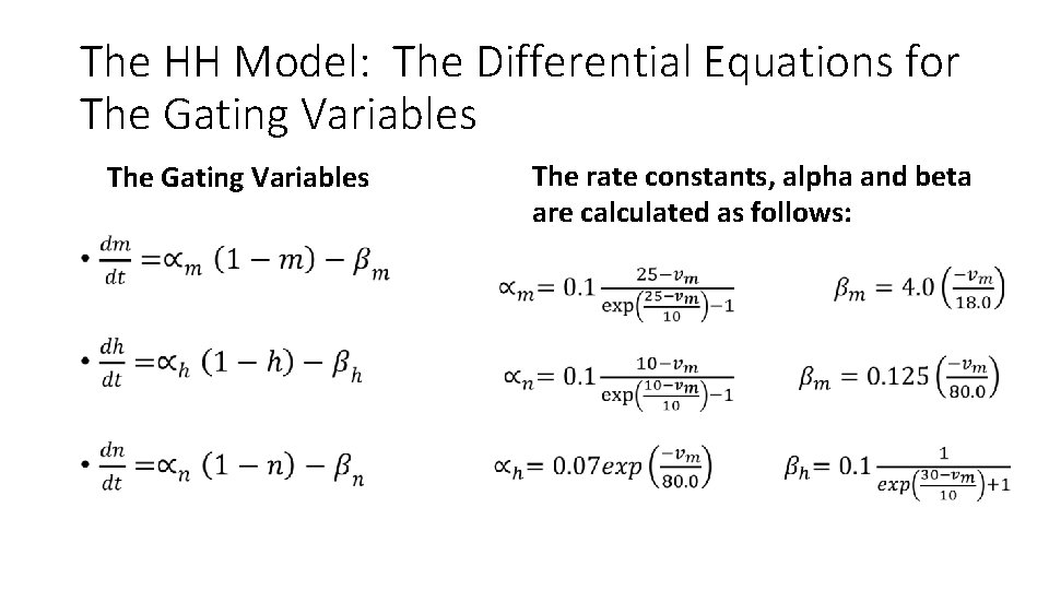
The HH Model: The Differential Equations for The Gating Variables • The rate constants, alpha and beta are calculated as follows:

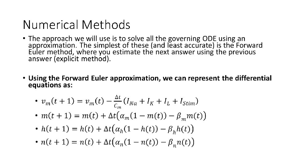
Numerical Methods •

Translate equations into MATLAB code function [outputv]=HH_Patch %INPUTS TOT_TIME=20; %ms dt=. 01; %Timestep in ms savedata=20; NTSTEPS=round(TOT_TIME/dt); %Number of Timesteps tvect=dt*[1: NTSTEPS]; %Time Vector %%%% SET THE STIMULUS PARAMETERS %%%% stimval=20; %u. A/cm 2 stimdur=2; %ms

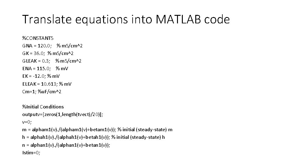
Translate equations into MATLAB code %CONSTANTS GNA = 120. 0; % m. S/cm^2 GK = 36. 0; % m. S/cm^2 GLEAK = 0. 3; % m. S/cm^2 ENA = 115. 0; % m. V EK = -12. 0; % m. V ELEAK = 10. 613; % m. V Cm=1; %u. F/cm^2 %Initial Conditions outputv=[zeros(1, length(tvect)/20)]; v=0; m = alpham 1(v). /(alpham 1(v)+betam 1(v)); % initial (steady-state) m h = alphah 1(v). /(alphah 1(v)+betah 1(v)); % initial (steady-state) h n = alphan 1(v). /(alphan 1(v)+betan 1(v)); Istim=0;

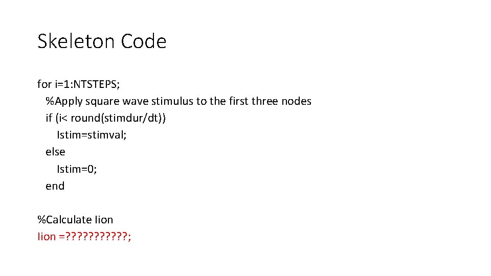
Skeleton Code for i=1: NTSTEPS; %Apply square wave stimulus to the first three nodes if (i< round(stimdur/dt)) Istim=stimval; else Istim=0; end %Calculate Iion =? ? ? ;

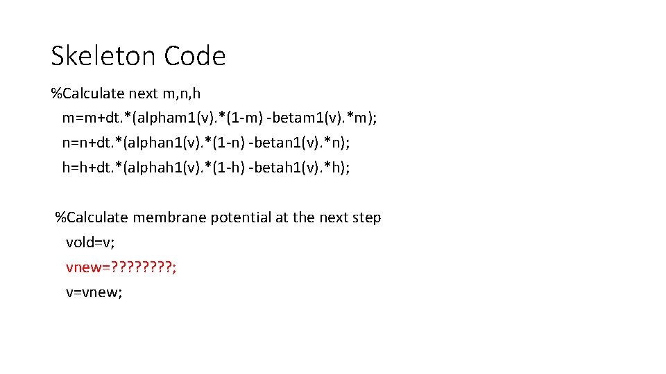
Skeleton Code %Calculate next m, n, h m=m+dt. *(alpham 1(v). *(1 -m) -betam 1(v). *m); n=n+dt. *(alphan 1(v). *(1 -n) -betan 1(v). *n); h=h+dt. *(alphah 1(v). *(1 -h) -betah 1(v). *h); %Calculate membrane potential at the next step vold=v; vnew=? ? ? ? ; v=vnew;

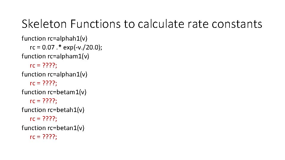
Skeleton Functions to calculate rate constants function rc=alphah 1(v) rc = 0. 07. * exp(-v. /20. 0); function rc=alpham 1(v) rc = ? ? ; function rc=alphan 1(v) rc = ? ? ; function rc=betam 1(v) rc = ? ? ; function rc=betah 1(v) rc = ? ? ; function rc=betan 1(v) rc = ? ? ;

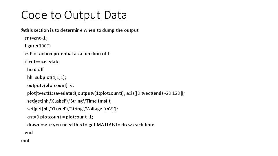
Code to Output Data %this section is to determine when to dump the output cnt=cnt+1; figure(1000) % Plot action potential as a function of t if cnt==savedata hold off hh=subplot(1, 1, 1); outputv(plotcount)=v; plot(tvect(1: savedata: i), outputv(1: plotcount)), axis([0 tvect(end) -20 120]); set(get(hh, 'XLabel'), 'String', 'Time (ms)'); set(get(hh, 'YLabel'), 'String', 'Voltage (m. V)'); cnt=0; plotcount = plotcount+1; drawnow % you need this to get MATLAB to draw each time end

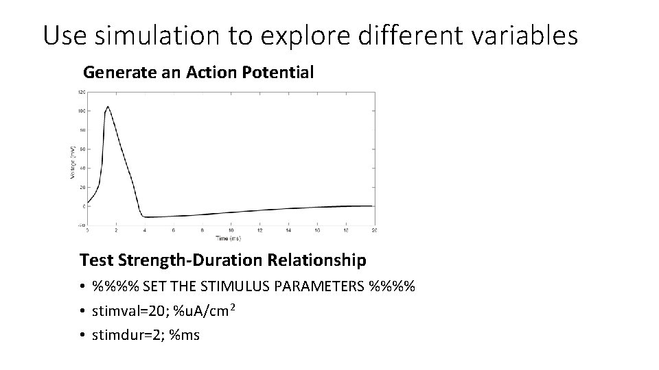
Use simulation to explore different variables Generate an Action Potential Test Strength-Duration Relationship • %%%% SET THE STIMULUS PARAMETERS %%%% • stimval=20; %u. A/cm 2 • stimdur=2; %ms