CPU Scheduling Scheduling the processor among all ready

CPU Scheduling • Scheduling the processor among all ready processes • The goal is to achieve: o High processor utilization o High throughput • number of processes completed per of unit time o Low response time • time elapsed from the submission of a request until the first response is produced • CPU Scheduling algorithms follows preemption and non preemption techniques. Footer Text 12/27/2021 1

Preemptive Vs Non Preemptive • In Pre-emptive scheduling the currently running process may be interrupted and moved to the ready state by OS (forcefully) • In Non-preemptive Scheduling, the running process can only lose the processor voluntarily by terminating or by requesting an I/O. OR, Once CPU given to a process it cannot be preempted until the process completes its CPU burst Footer Text 12/27/2021 2

CPU Scheduling Algorithms • • First Come First Serve Shortest Job First Shortest Remaining Time First Priority Scheduling Round Robin High Response Ratio Time First Multilevel Queue Scheduling Multilevel Feedback Queue Scheduling Footer Text 12/27/2021 3

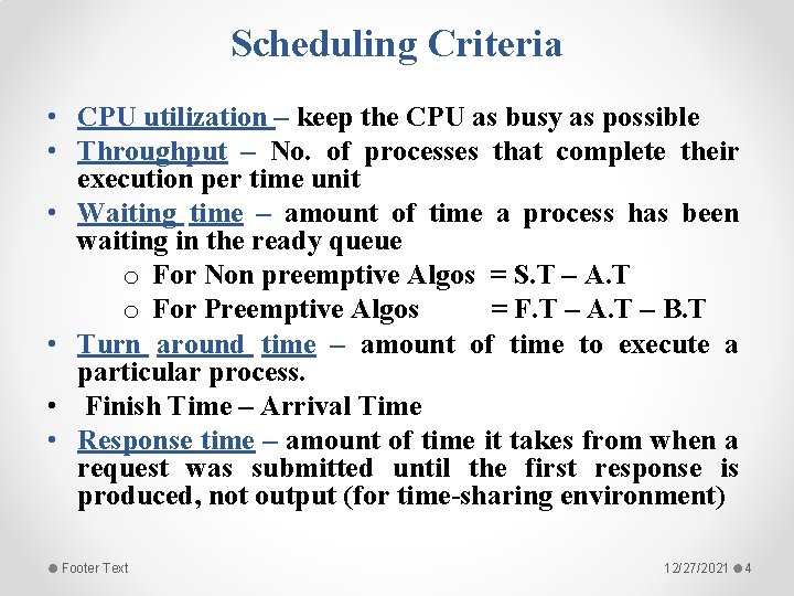
Scheduling Criteria • CPU utilization – keep the CPU as busy as possible • Throughput – No. of processes that complete their execution per time unit • Waiting time – amount of time a process has been waiting in the ready queue o For Non preemptive Algos = S. T – A. T o For Preemptive Algos = F. T – A. T – B. T • Turn around time – amount of time to execute a particular process. • Finish Time – Arrival Time • Response time – amount of time it takes from when a request was submitted until the first response is produced, not output (for time-sharing environment) Footer Text 12/27/2021 4

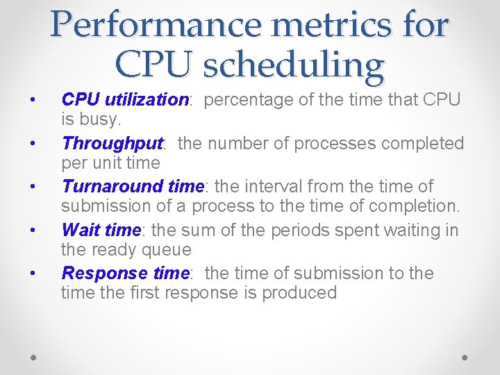
Performance metrics for CPU scheduling • • • CPU utilization: percentage of the time that CPU is busy. Throughput: the number of processes completed per unit time Turnaround time: the interval from the time of submission of a process to the time of completion. Wait time: the sum of the periods spent waiting in the ready queue Response time: the time of submission to the time the first response is produced

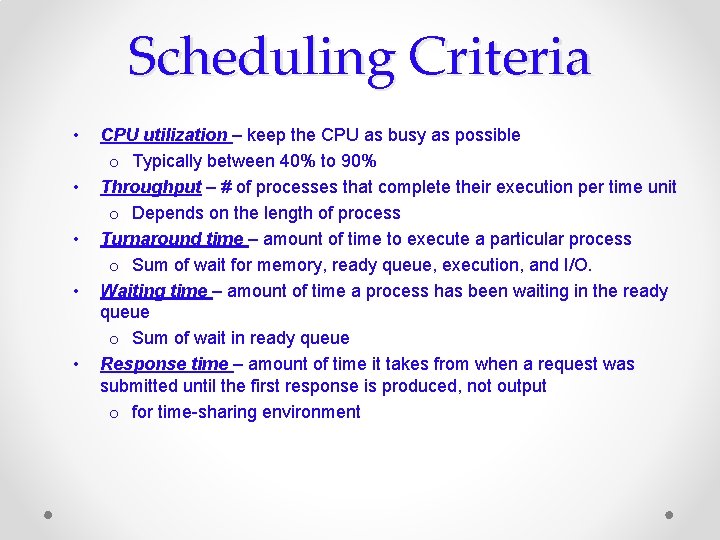
Scheduling Criteria • • • CPU utilization – keep the CPU as busy as possible o Typically between 40% to 90% Throughput – # of processes that complete their execution per time unit o Depends on the length of process Turnaround time – amount of time to execute a particular process o Sum of wait for memory, ready queue, execution, and I/O. Waiting time – amount of time a process has been waiting in the ready queue o Sum of wait in ready queue Response time – amount of time it takes from when a request was submitted until the first response is produced, not output o for time-sharing environment

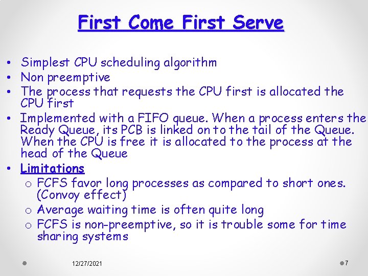
First Come First Serve • Simplest CPU scheduling algorithm • Non preemptive • The process that requests the CPU first is allocated the CPU first • Implemented with a FIFO queue. When a process enters the Ready Queue, its PCB is linked on to the tail of the Queue. When the CPU is free it is allocated to the process at the head of the Queue • Limitations o FCFS favor long processes as compared to short ones. (Convoy effect) o Average waiting time is often quite long o FCFS is non-preemptive, so it is trouble some for time sharing systems 12/27/2021 7

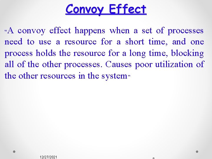
Convoy Effect A convoy effect happens when a set of processes need to use a resource for a short time, and one process holds the resource for a long time, blocking all of the other processes. Causes poor utilization of the other resources in the system” “ 12/27/2021

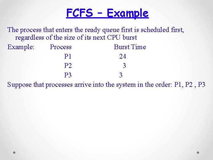
FCFS – Example The process that enters the ready queue first is scheduled first, regardless of the size of its next CPU burst Example: Process Burst Time P 1 24 P 2 3 P 3 3 Suppose that processes arrive into the system in the order: P 1, P 2 , P 3

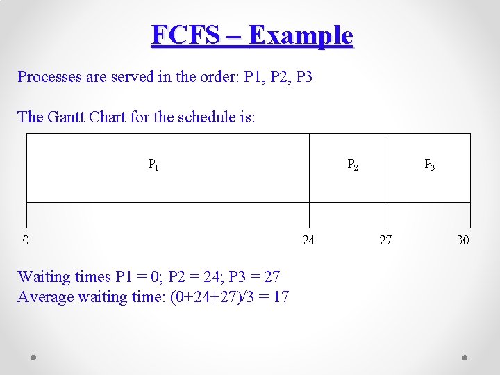
FCFS – Example Processes are served in the order: P 1, P 2, P 3 The Gantt Chart for the schedule is: P 1 0 Waiting times P 1 = 0; P 2 = 24; P 3 = 27 Average waiting time: (0+24+27)/3 = 17 P 2 24 P 3 27 30

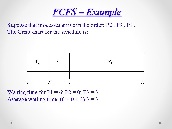
FCFS – Example Suppose that processes arrive in the order: P 2 , P 3 , P 1. The Gantt chart for the schedule is: P 2 0 P 3 3 P 1 6 Waiting time for P 1 = 6; P 2 = 0; P 3 = 3 Average waiting time: (6 + 0 + 3)/3 = 3 30

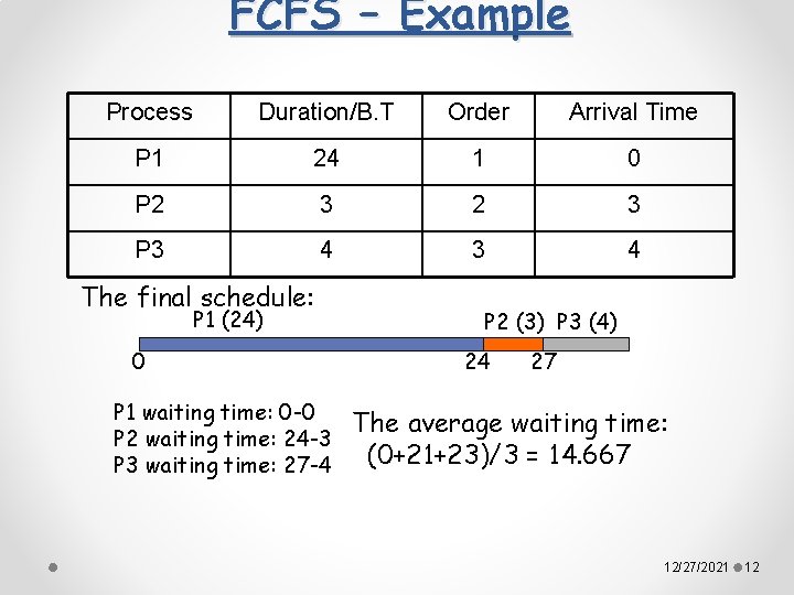
FCFS – Example Process Duration/B. T Order Arrival Time P 1 24 1 0 P 2 3 P 3 4 The final schedule: P 1 (24) 0 P 1 waiting time: 0 -0 P 2 waiting time: 24 -3 P 3 waiting time: 27 -4 P 2 (3) P 3 (4) 24 27 The average waiting time: (0+21+23)/3 = 14. 667 12/27/2021 12

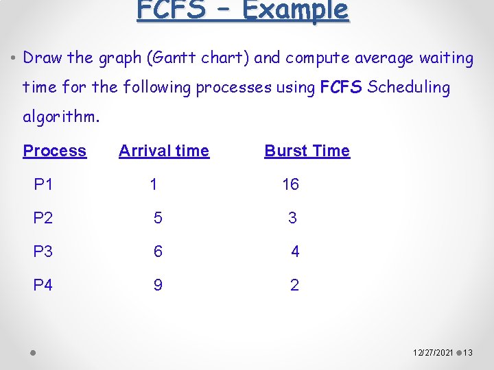
FCFS – Example • Draw the graph (Gantt chart) and compute average waiting time for the following processes using FCFS Scheduling algorithm. Process Arrival time Burst Time P 1 1 16 P 2 5 3 P 3 6 4 P 4 9 2 12/27/2021 13

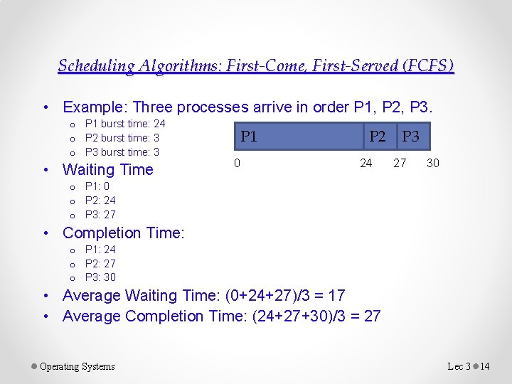
Scheduling Algorithms: First-Come, First-Served (FCFS) • Example: Three processes arrive in order P 1, P 2, P 3. o P 1 burst time: 24 o P 2 burst time: 3 o P 3 burst time: 3 • Waiting Time P 1 0 P 2 24 P 3 27 30 o P 1: 0 o P 2: 24 o P 3: 27 • Completion Time: o P 1: 24 o P 2: 27 o P 3: 30 • Average Waiting Time: (0+24+27)/3 = 17 • Average Completion Time: (24+27+30)/3 = 27 Operating Systems Lec 3 14

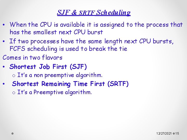
SJF & SRTF Scheduling • When the CPU is available it is assigned to the process that has the smallest next CPU burst • If two processes have the same length next CPU bursts, FCFS scheduling is used to break the tie Comes in two flavors • Shortest Job First (SJF) o It’s a non preemptive algorithm. • Shortest Remaining Time First (SRTF) o It’s a Preemptive algorithm. 12/27/2021 15

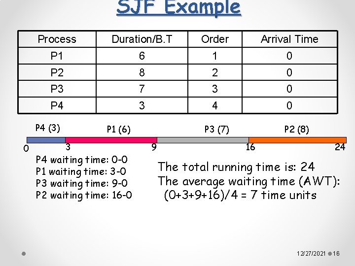
SJF Example Process Duration/B. T Order Arrival Time P 1 6 1 0 P 2 8 2 0 P 3 7 3 0 P 4 3 4 0 P 4 (3) 0 P 1 (6) 3 P 4 waiting time: 0 -0 P 1 waiting time: 3 -0 P 3 waiting time: 9 -0 P 2 waiting time: 16 -0 P 3 (7) 9 P 2 (8) 16 24 The total running time is: 24 The average waiting time (AWT): (0+3+9+16)/4 = 7 time units 12/27/2021 16

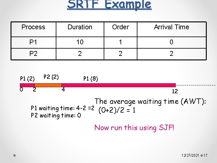
SRTF Example Process Duration Order Arrival Time P 1 10 1 0 P 2 2 P 1 (2) 0 2 P 2 (2) P 1 (8) 4 12 The average waiting time (AWT): P 1 waiting time: 4 -2 =2 (0+2)/2 = 1 P 2 waiting time: 0 Now run this using SJF! 12/27/2021 17

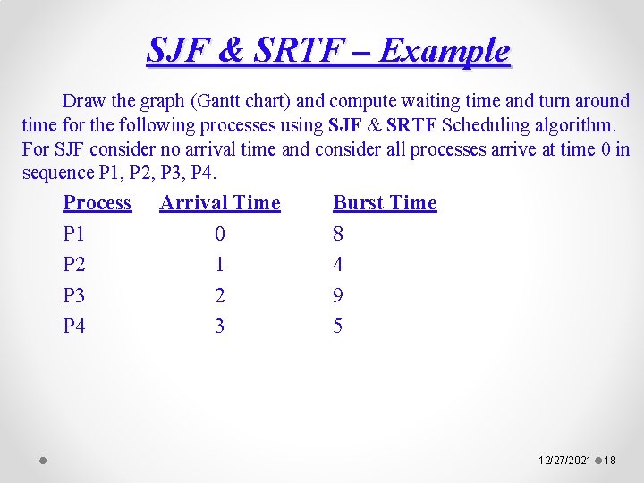
SJF & SRTF – Example Draw the graph (Gantt chart) and compute waiting time and turn around time for the following processes using SJF & SRTF Scheduling algorithm. For SJF consider no arrival time and consider all processes arrive at time 0 in sequence P 1, P 2, P 3, P 4. Process P 1 P 2 P 3 P 4 Arrival Time 0 1 2 3 Burst Time 8 4 9 5 12/27/2021 18

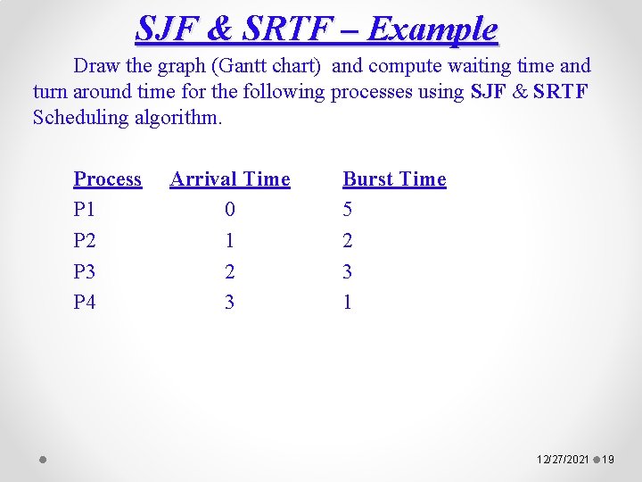
SJF & SRTF – Example Draw the graph (Gantt chart) and compute waiting time and turn around time for the following processes using SJF & SRTF Scheduling algorithm. Process P 1 P 2 P 3 P 4 Arrival Time 0 1 2 3 Burst Time 5 2 3 1 12/27/2021 19

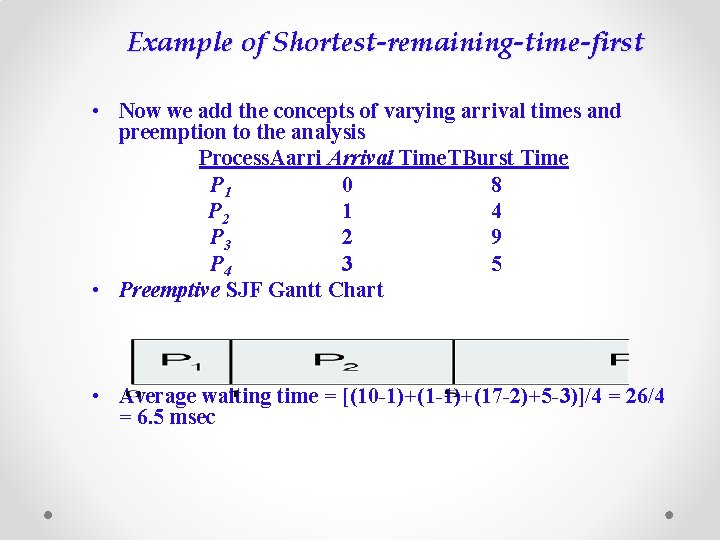
Example of Shortest-remaining-time-first • Now we add the concepts of varying arrival times and preemption to the analysis Process. Aarri Arrival Time. TBurst Time P 1 0 8 P 2 1 4 P 3 2 9 P 4 3 5 • Preemptive SJF Gantt Chart • Average waiting time = [(10 -1)+(17 -2)+5 -3)]/4 = 26/4 = 6. 5 msec

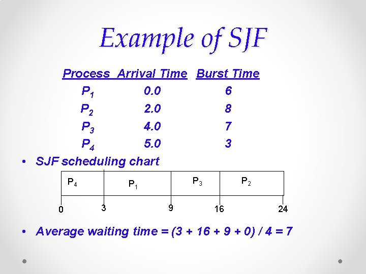
Example of SJF Process Arrival Time Burst Time P 1 0. 0 6 P 2 2. 0 8 P 3 4. 0 7 P 4 5. 0 3 • SJF scheduling chart P 4 0 P 3 P 1 3 9 P 2 16 24 • Average waiting time = (3 + 16 + 9 + 0) / 4 = 7

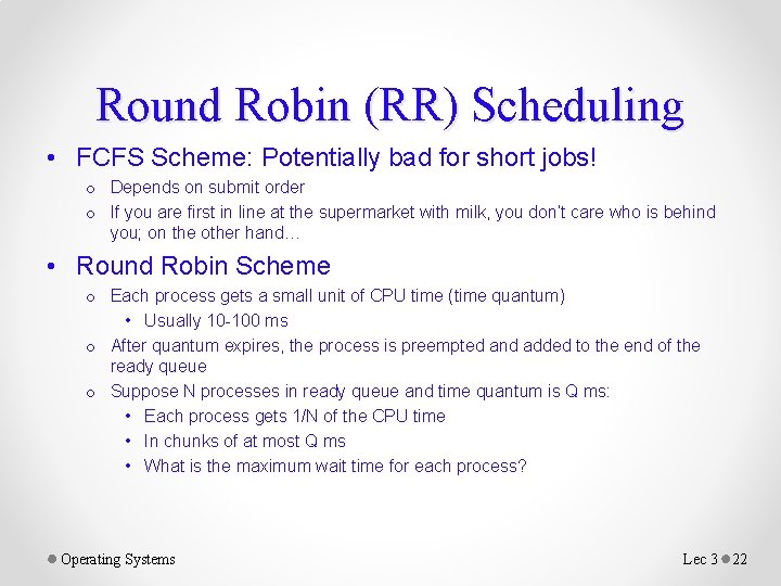
Round Robin (RR) Scheduling • FCFS Scheme: Potentially bad for short jobs! o Depends on submit order o If you are first in line at the supermarket with milk, you don’t care who is behind you; on the other hand… • Round Robin Scheme o Each process gets a small unit of CPU time (time quantum) • Usually 10 -100 ms o After quantum expires, the process is preempted and added to the end of the ready queue o Suppose N processes in ready queue and time quantum is Q ms: • Each process gets 1/N of the CPU time • In chunks of at most Q ms • What is the maximum wait time for each process? Operating Systems Lec 3 22

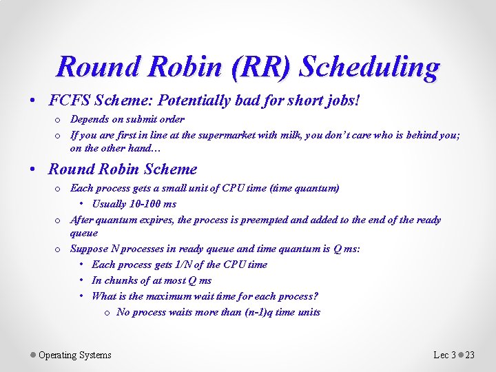
Round Robin (RR) Scheduling • FCFS Scheme: Potentially bad for short jobs! o Depends on submit order o If you are first in line at the supermarket with milk, you don’t care who is behind you; on the other hand… • Round Robin Scheme o Each process gets a small unit of CPU time (time quantum) • Usually 10 -100 ms o After quantum expires, the process is preempted and added to the end of the ready queue o Suppose N processes in ready queue and time quantum is Q ms: • Each process gets 1/N of the CPU time • In chunks of at most Q ms • What is the maximum wait time for each process? o No process waits more than (n-1)q time units Operating Systems Lec 3 23

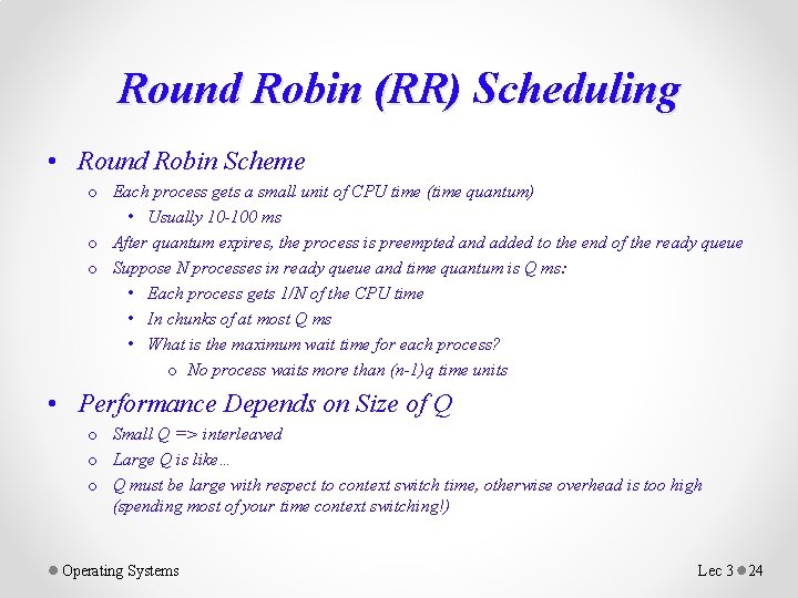
Round Robin (RR) Scheduling • Round Robin Scheme o Each process gets a small unit of CPU time (time quantum) • Usually 10 -100 ms o After quantum expires, the process is preempted and added to the end of the ready queue o Suppose N processes in ready queue and time quantum is Q ms: • Each process gets 1/N of the CPU time • In chunks of at most Q ms • What is the maximum wait time for each process? o No process waits more than (n-1)q time units • Performance Depends on Size of Q o Small Q => interleaved o Large Q is like… o Q must be large with respect to context switch time, otherwise overhead is too high (spending most of your time context switching!) Operating Systems Lec 3 24

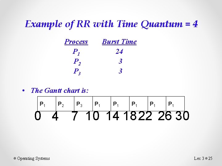
Example of RR with Time Quantum = 4 Process P 1 P 2 P 3 Burst Time 24 3 3 • The Gantt chart is: P 1 P 2 P 3 P 1 P 1 P 1 0 4 7 10 14 1822 26 30 Operating Systems Lec 3 25

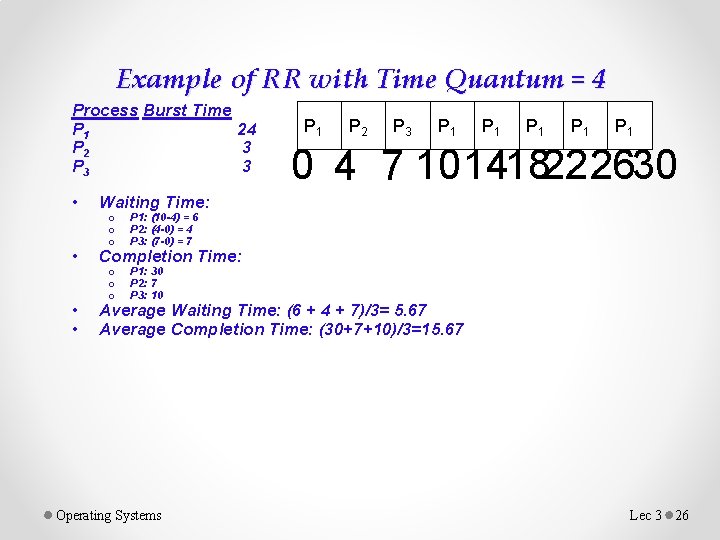
Example of RR with Time Quantum = 4 Process Burst Time P 1 24 P 2 3 P 3 3 P 1 P 2 P 3 P 1 Waiting Time: • Completion Time: • • Average Waiting Time: (6 + 4 + 7)/3= 5. 67 Average Completion Time: (30+7+10)/3=15. 67 P 1: (10 -4) = 6 P 2: (4 -0) = 4 P 3: (7 -0) = 7 o o o P 1: 30 P 2: 7 P 3: 10 Operating Systems P 1 P 1 0 4 7 101418222630 • o o o P 1 Lec 3 26

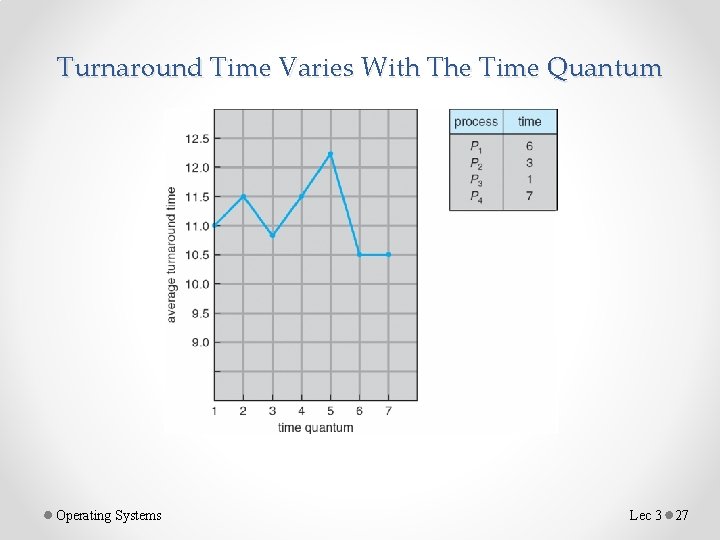
Turnaround Time Varies With The Time Quantum Operating Systems Lec 3 27

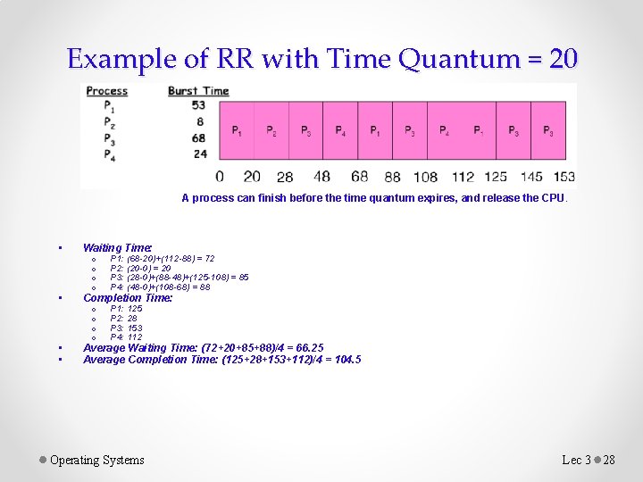
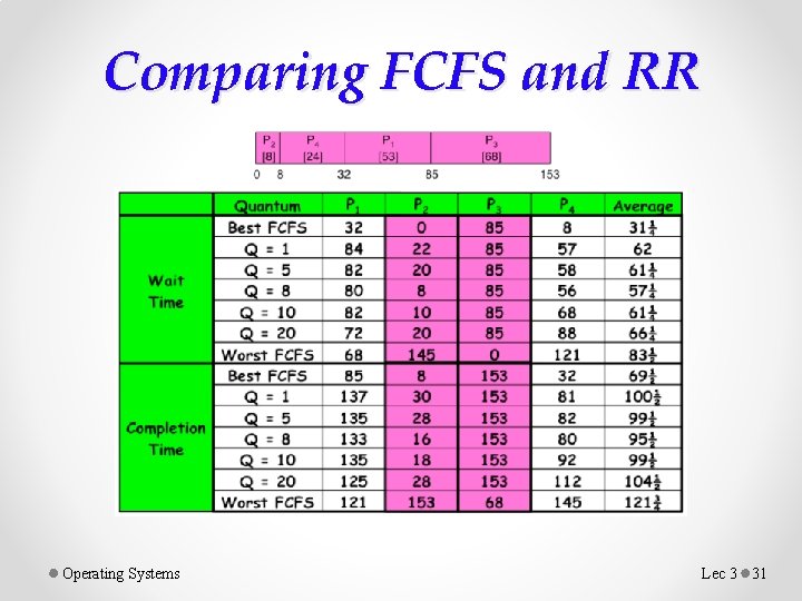
Example of RR with Time Quantum = 20 A process can finish before the time quantum expires, and release the CPU. • Waiting Time: • Completion Time: • • Average Waiting Time: (72+20+85+88)/4 = 66. 25 Average Completion Time: (125+28+153+112)/4 = 104. 5 o o P 1: (68 -20)+(112 -88) = 72 P 2: (20 -0) = 20 P 3: (28 -0)+(88 -48)+(125 -108) = 85 P 4: (48 -0)+(108 -68) = 88 o o P 1: 125 P 2: 28 P 3: 153 P 4: 112 Operating Systems Lec 3 28

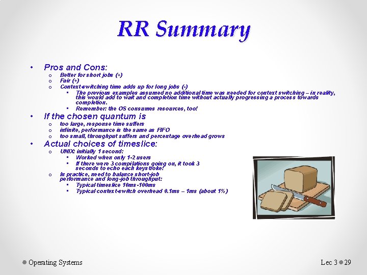
RR Summary • Pros and Cons: • If the chosen quantum is • Actual choices of timeslice: o o o Better for short jobs (+) Fair (+) Context-switching time adds up for long jobs (-) • The previous examples assumed no additional time was needed for context switching – in reality, this would add to wait and completion time without actually progressing a process towards completion. • Remember: the OS consumes resources, too! o o o too large, response time suffers infinite, performance is the same as FIFO too small, throughput suffers and percentage overhead grows o UNIX: initially 1 second: • Worked when only 1 -2 users • If there were 3 compilations going on, it took 3 seconds to echo each keystroke! In practice, need to balance short-job performance and long-job throughput: • Typical timeslice 10 ms-100 ms • Typical context-switch overhead 0. 1 ms – 1 ms (about 1%) o Operating Systems Lec 3 29

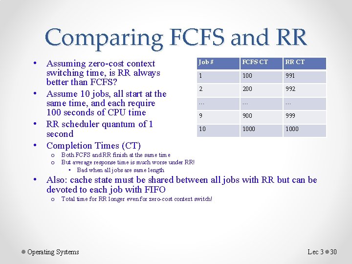
Comparing FCFS and RR • Assuming zero-cost context switching time, is RR always better than FCFS? • Assume 10 jobs, all start at the same time, and each require 100 seconds of CPU time • RR scheduler quantum of 1 second • Completion Times (CT) o o Job # FCFS CT RR CT 1 100 991 2 200 992 … … … 9 900 999 10 1000 Both FCFS and RR finish at the same time But average response time is much worse under RR! • Bad when all jobs are same length • Also: cache state must be shared between all jobs with RR but can be devoted to each job with FIFO o Total time for RR longer even for zero-cost context switch! Operating Systems Lec 3 30

Comparing FCFS and RR Operating Systems Lec 3 31

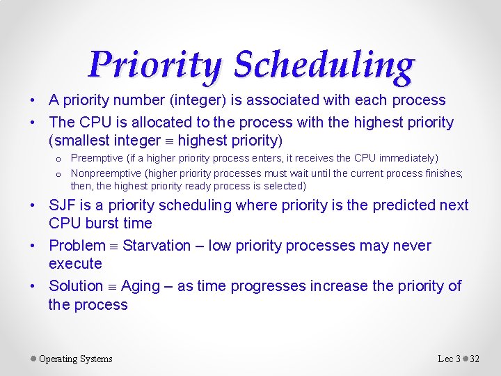
Priority Scheduling • A priority number (integer) is associated with each process • The CPU is allocated to the process with the highest priority (smallest integer highest priority) o Preemptive (if a higher priority process enters, it receives the CPU immediately) o Nonpreemptive (higher priority processes must wait until the current process finishes; then, the highest priority ready process is selected) • SJF is a priority scheduling where priority is the predicted next CPU burst time • Problem Starvation – low priority processes may never execute • Solution Aging – as time progresses increase the priority of the process Operating Systems Lec 3 32

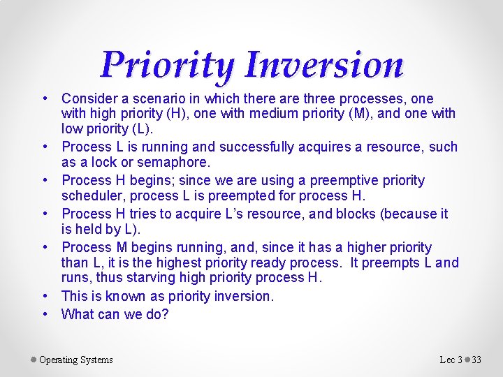
Priority Inversion • Consider a scenario in which there are three processes, one with high priority (H), one with medium priority (M), and one with low priority (L). • Process L is running and successfully acquires a resource, such as a lock or semaphore. • Process H begins; since we are using a preemptive priority scheduler, process L is preempted for process H. • Process H tries to acquire L’s resource, and blocks (because it is held by L). • Process M begins running, and, since it has a higher priority than L, it is the highest priority ready process. It preempts L and runs, thus starving high priority process H. • This is known as priority inversion. • What can we do? Operating Systems Lec 3 33

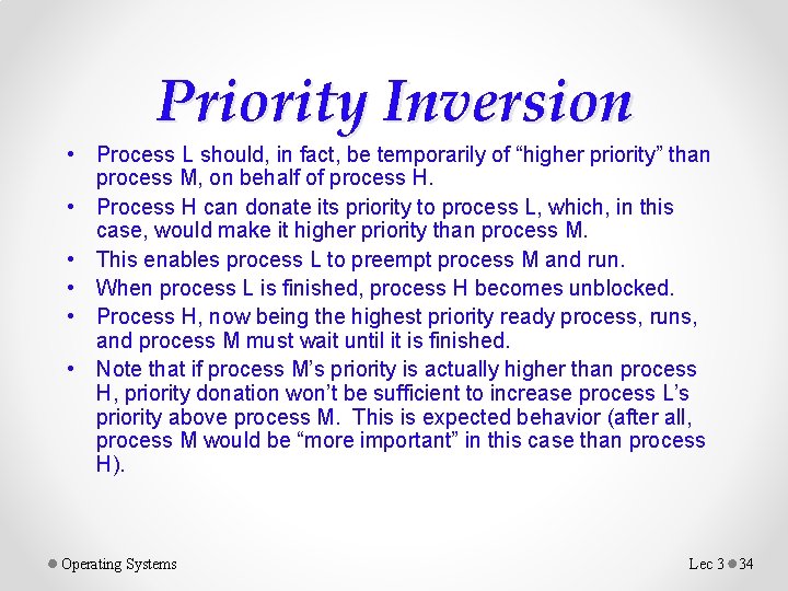
Priority Inversion • Process L should, in fact, be temporarily of “higher priority” than process M, on behalf of process H. • Process H can donate its priority to process L, which, in this case, would make it higher priority than process M. • This enables process L to preempt process M and run. • When process L is finished, process H becomes unblocked. • Process H, now being the highest priority ready process, runs, and process M must wait until it is finished. • Note that if process M’s priority is actually higher than process H, priority donation won’t be sufficient to increase process L’s priority above process M. This is expected behavior (after all, process M would be “more important” in this case than process H). Operating Systems Lec 3 34

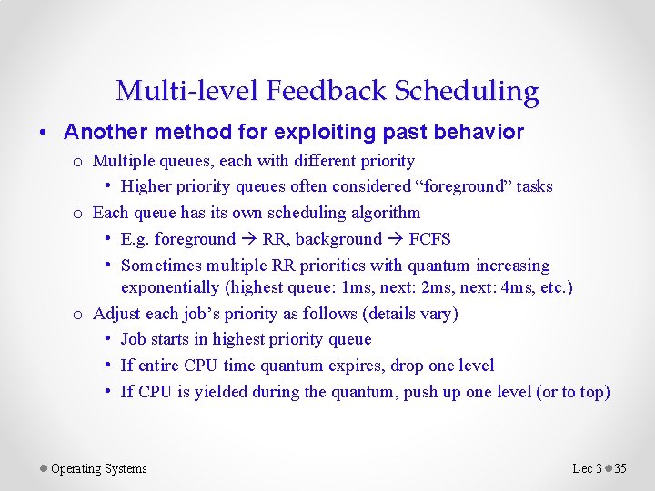
Multi-level Feedback Scheduling • Another method for exploiting past behavior o Multiple queues, each with different priority • Higher priority queues often considered “foreground” tasks o Each queue has its own scheduling algorithm • E. g. foreground RR, background FCFS • Sometimes multiple RR priorities with quantum increasing exponentially (highest queue: 1 ms, next: 2 ms, next: 4 ms, etc. ) o Adjust each job’s priority as follows (details vary) • Job starts in highest priority queue • If entire CPU time quantum expires, drop one level • If CPU is yielded during the quantum, push up one level (or to top) Operating Systems Lec 3 35

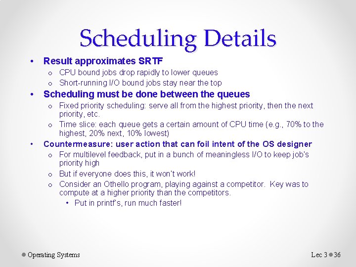
Scheduling Details • Result approximates SRTF o CPU bound jobs drop rapidly to lower queues o Short-running I/O bound jobs stay near the top • • Scheduling must be done between the queues o Fixed priority scheduling: serve all from the highest priority, then the next priority, etc. o Time slice: each queue gets a certain amount of CPU time (e. g. , 70% to the highest, 20% next, 10% lowest) Countermeasure: user action that can foil intent of the OS designer o For multilevel feedback, put in a bunch of meaningless I/O to keep job’s priority high o But if everyone does this, it won’t work! o Consider an Othello program, playing against a competitor. Key was to compute at a higher priority than the competitors. • Put in printf’s, run much faster! Operating Systems Lec 3 36

Scheduling Details • It is apparent that scheduling is facilitated by having a “good mix” of I/O bound and CPU bound programs, so that there are long and short CPU bursts to prioritize around. • There is typically a long-term and a short-term scheduler in the OS. • We have been discussing the design of the short-term scheduler. • The long-term scheduler decides what processes should be put into the ready queue in the first place for the short-term scheduler, so that the short-term scheduler can make fast decisions on a good mix of a subset of ready processes. • The rest are held in memory or disk o Why else is this helpful? Operating Systems Lec 3 37

Scheduling Details • • • It is apparent that scheduling is facilitated by having a “good mix” of I/O bound and CPU bound programs, so that there are long and short CPU bursts to prioritize around. There is typically a long-term and a short-term scheduler in the OS. We have been discussing the design of the short-term scheduler. The long-term scheduler decides what processes should be put into the ready queue in the first place for the short-term scheduler, so that the short-term scheduler can make fast decisions on a good mix of a subset of ready processes. The rest are held in memory or disk o This also provides more free memory for the subset of ready processes given to the short-term scheduler. Operating Systems Lec 3 38

Fairness • What about fairness? o Strict fixed-policy scheduling between queues is unfair (run highest, then next, etc. ) • Long running jobs may never get the CPU • In Multics, admins shut down the machine and found a 10 -year-old job o Must give long-running jobs a fraction of the CPU even when there are shorter jobs to run • Tradeoff: fairness gained by hurting average response time! • How to implement fairness? o o Could give each queue some fraction of the CPU • i. e. , for one long-running job and 100 short-running ones? • Like express lanes in a supermarket – sometimes express lanes get so long, one gets better service by going into one of the regular lines Could increase priority of jobs that don’t get service (as seen in the multilevel feedback example) • This was done in UNIX • Ad hoc – with what rate should priorities be increased? • As system gets overloaded, no job gets CPU time, so everyone increases in priority o Interactive processes suffer Operating Systems Lec 3 39

Lottery Scheduling • Yet another alternative: Lottery Scheduling o Give each job some number of lottery tickets o On each time slice, randomly pick a winning ticket o On average, CPU time is proportional to number of tickets given to each job over time • How to assign tickets? o To approximate SRTF, short-running jobs get more, long running jobs get fewer o To avoid starvation, every job gets at least one ticket (everyone makes progress) • Advantage over strict priority scheduling: behaves gracefully as load changes o Adding or deleting a job affects all jobs proportionally, independent of how many tickets each job possesses Operating Systems Lec 3 40

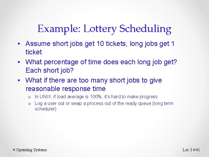
Example: Lottery Scheduling • Assume short jobs get 10 tickets, long jobs get 1 ticket • What percentage of time does each long job get? Each short job? • What if there are too many short jobs to give reasonable response time o In UNIX, if load average is 100%, it’s hard to make progress o Log a user out or swap a process out of the ready queue (long term scheduler) Operating Systems Lec 3 41

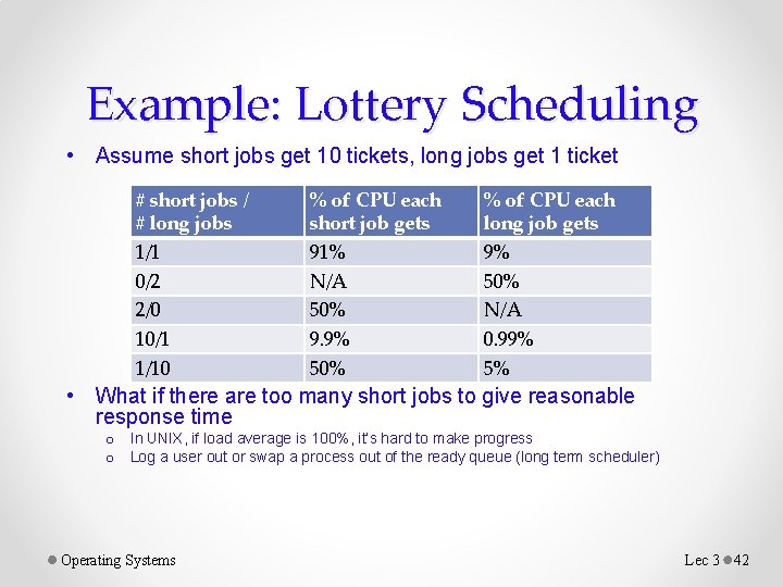
Example: Lottery Scheduling • Assume short jobs get 10 tickets, long jobs get 1 ticket # short jobs / # long jobs 1/1 0/2 2/0 10/1 1/10 % of CPU each short job gets 91% N/A 50% 9. 9% 50% % of CPU each long job gets 9% 50% N/A 0. 99% 5% • What if there are too many short jobs to give reasonable response time o In UNIX, if load average is 100%, it’s hard to make progress o Log a user out or swap a process out of the ready queue (long term scheduler) Operating Systems Lec 3 42

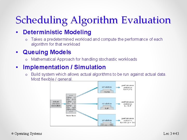
Scheduling Algorithm Evaluation • Deterministic Modeling o Takes a predetermined workload and compute the performance of each algorithm for that workload • Queuing Models o Mathematical Approach for handling stochastic workloads • Implementation / Simulation o Build system which allows actual algorithms to be run against actual data. Most flexible / general. Operating Systems Lec 3 43

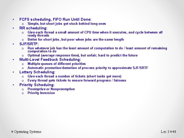
• • FCFS scheduling, FIFO Run Until Done: o RR scheduling: o • • Give each thread a small amount of CPU time when it executes, and cycle between all ready threads Better for short jobs, but poor when jobs are the same length SJF/SRTF: o • Simple, but short jobs get stuck behind long ones o Run whatever job has the least amount of computation to do / least amount of remaining computation to do Optimal (average response time), but unfair; hard to predict the future Multi-Level Feedback Scheduling: o o Multiple queues of different priorities Automatic promotion/demotion of process priority to approximate SJF/SRTF Lottery Scheduling: o o Give each thread a number of tickets (short tasks get more) Every thread gets tickets to ensure forward progress / fairness Priority Scheduing: o o Preemptive or Nonpreemptive Priority Inversion Operating Systems Lec 3 44