CPU Scheduling G Anuradha References Galvin and William

CPU Scheduling G. Anuradha References : Galvin and William Stallings Problems taken from Principles of OS by Naresh Chauhan

Objectives • To introduce CPU scheduling, which is the basis for multiprogrammed operating systems. • To describe various CPU-scheduling algorithms. • To discuss evaluation criteria for selecting a CPU-scheduling algorithm for a particular system. • To examine the scheduling algorithms of several operating systems.

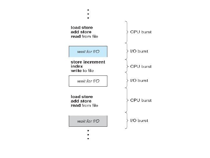
Basic concepts-CPU –I/O Burst cycle • Why Multi programming? – To Maximize CPU utilization • CPU Scheduling is central to OS design • For proper CPU scheduling the histogram of CPU-Burst duration is considered.

Frequency for shorter duration is much more than the frequency of longer duration This is the general trend

Types of Scheduler • Long-term Scheduler: -Needed only in the case of batch processing and is absent in multi user timesharing system. In time-sharing systems the jobs are directly entered into ready queue. • Short-term Scheduler: -Invoked whenever there is an interrupt, to select another process for execution. • Medium-term Scheduler: - Invoked when there is a need to swap out some blocked processes from memory to secondary storage.

Preemptive Scheduling • Circumstances when CPU-Scheduling Decisions may take place Preemptive Scheduling – Process switches from running state to waiting state (I/O, termination of child process) – Process switches from running to ready state(interrupt) – Process switches from waiting state to ready state(Completion of I/O) – Process terminates Non Preemptive Scheduling

What are the factors affecting preemptive scheduling? • Cost associated with access to shared data. Cooperative process • Affects the design of os kernel

Role of dispatcher • Switching context • Switching to user mode • Jumping to the proper location in the user program to restart the program Dispatch Latency is the time taken to stop one process and start another running process.

Scheduling Criteria • CPU Utilization • Throughput: Number of processes completed per unit time • Turnaround time: the interval from the time of submission of a process to the time of completion • Turnaround time= waiting time+ execution time

• Waiting time: sum of periods spend waiting in the ready queue • Response time: - time taken to start responding • Maximize CPU utilization, Maximize throughput, minimize turnaround time, waiting time and response time.

Scheduling Algorithms • • • First Cum First Served Scheduling(FCFS) Shortest job First(SJF) Shortest Remaining Time Next(SRTN) Round Robin(RR) Multilevel Queue Scheduling

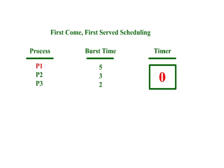
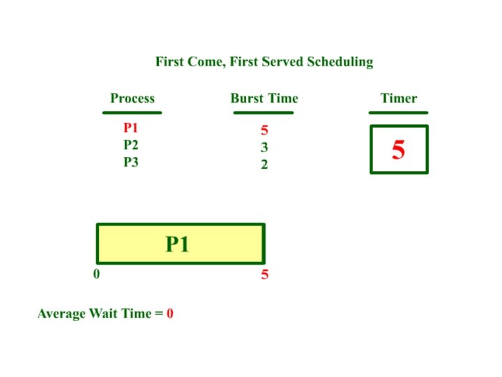
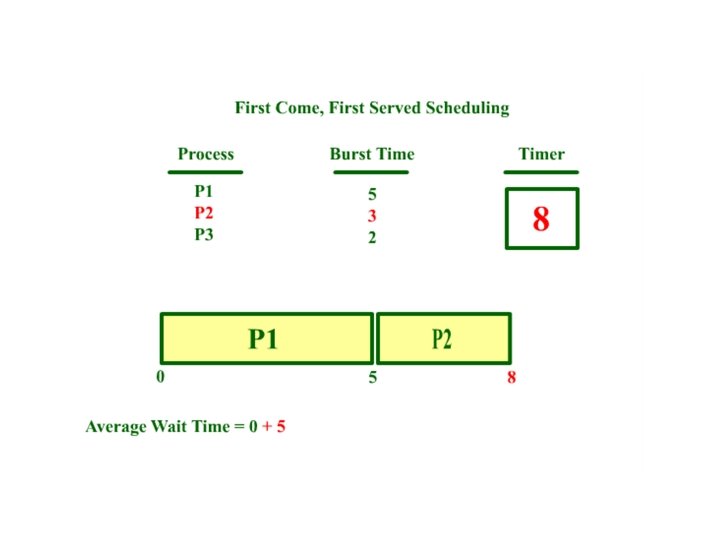
First Cum First Served (FCFS)

If process come in the order P 3, P 2, P 1 find the average waiting time.

Waiting time for P 1=0 Average Execution time=(5+3+2)/3=3. 33 Waiting time for P 2=5 Waiting time for P 3=8 Average Waiting time=(0+5+8)/3=4. 33 Average Turn Around time=Average Waiting time + Average Execution time =4. 33+3. 33 =7. 66 Average Response time=(0+5+8)/3=4. 33

Features of FCFS • Average waiting time under FSFS varies if the CPU burst times vary greatly • Convey effect is produced because of CPU and IO bound processes • FCFS is non preemptive.

Solve Average Waiting time Average Execution time Average Turn Around time Average Response time

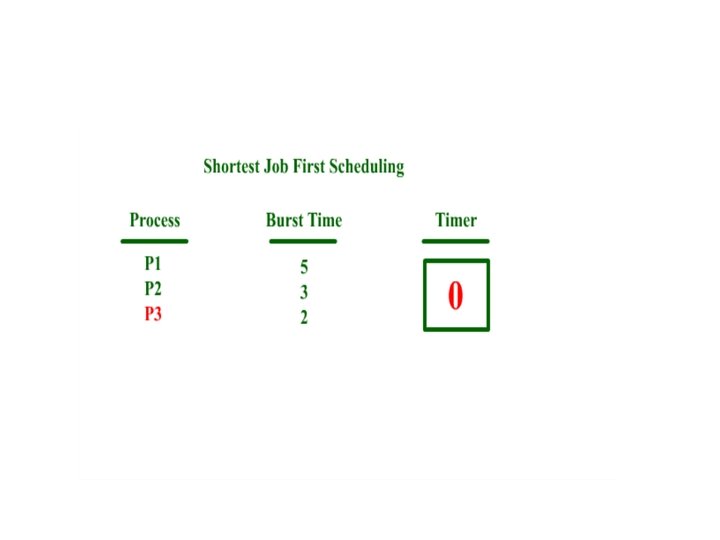
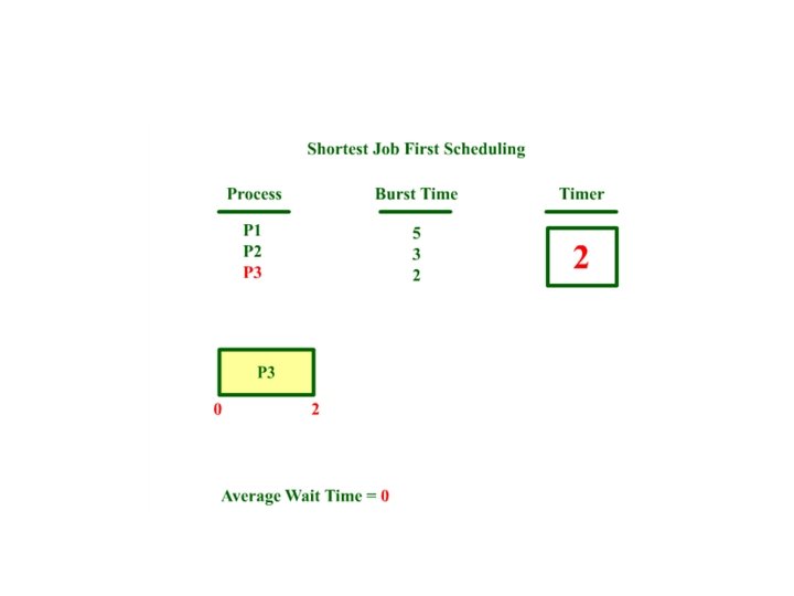
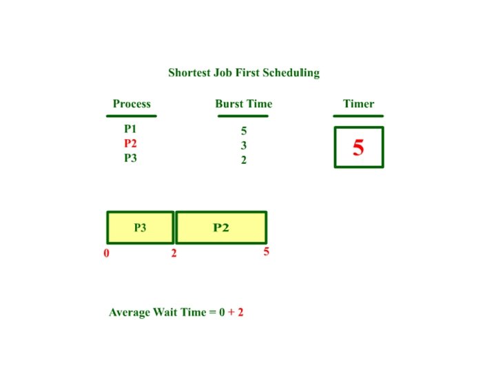
Shortest Job First

Average Execution time=(5+3+2)/3=3. 33 Average Turn Around Time=3. 33+2. 33=5. 66 Average Response time=(0+2+5)/3=2. 33

Solve Average Waiting time Average Execution time Average Turn Around time Average Response time

Difficulties in SJF algorithm • Optimal. The length of the next CPU request is not known in advance • The burst time of the next process can be predicted. The predicted value for the next CPU burst is depended on recent information tn and past history SJF can be preemptive or nonpreemptive. Preemptive SJF is called as Shortest remaining time first scheduling

Shortest Remaining Time First Scheduling P 1 0 Process Arrival Time Burst Time P 1 0 8 P 2 1 4 P 3 2 9 P 4 3 5 P 2 1 P 4 5 P 1 10 WT of P 1=(10 -1)=9 WT of P 2=0 WT of P 3=(17 -2)=15 WT of P 4=(5 -3)=2 Average WT=(9+0+15+2)/4=6. 5 ms Average Execution Time=(8+4+9+5)/5=6. 5 ATAT=6. 5+6. 5=13 ms P 3 17 26

STF Process Arrival Time Burst Time P 1 0 8 P 2 1 4 P 3 2 9 P 4 3 5 P 1 0 P 2 8 P 4 12 WT for P 1=0 WT for P 2=(8 -1)=7 WT for P 3=(17 -2)=15 WT for P 4=(12 -3)=9 Average WT=(0+7+15+9)/4=7. 75 ATAT=6. 5+7. 75=14. 25 ms P 3 17 26

Solve(SJF and SRTF) Process Arrival Time Burst Time P 1 0 9 P 2 1 5 P 3 2 3 P 4 3 4

Priority Scheduling All process arrive at time t=0 P 2 0 Process Burst Time Priority P 1 10 3 P 2 1 1 P 3 2 4 P 4 1 5 P 5 5 2 P 5 1 P 1 6 P 3 16 P 4 18 19

Priority Scheduling All process arrive at time t=0 Process Burst Time Priority WT TT Normalized TT P 1 10 3 6 16 1. 6 P 2 1 1 0 1 1 P 3 2 4 16 18 9 P 4 1 5 18 19 19 P 5 5 2 1 6 1. 2 8. 2 12 6. 36 3. 8

Priority Scheduling(PS) Contd… • PS can be – Internal: use measurable quantity to compute priority, like time limits, memory requirements, number of open files, etc. – External: Importance of process, type and amount of funds paid for computer use • PS can be either – Preemptive: – Non Preemptive:

Starvation • Why starvation happens? – When low priority job waits indefinitely • Solution to starvation is aging – Increasing the priority of processes that wait in the system for long time

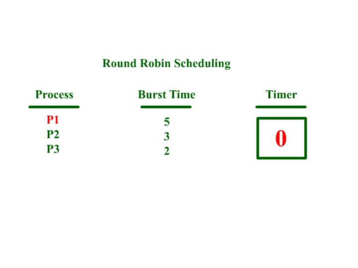
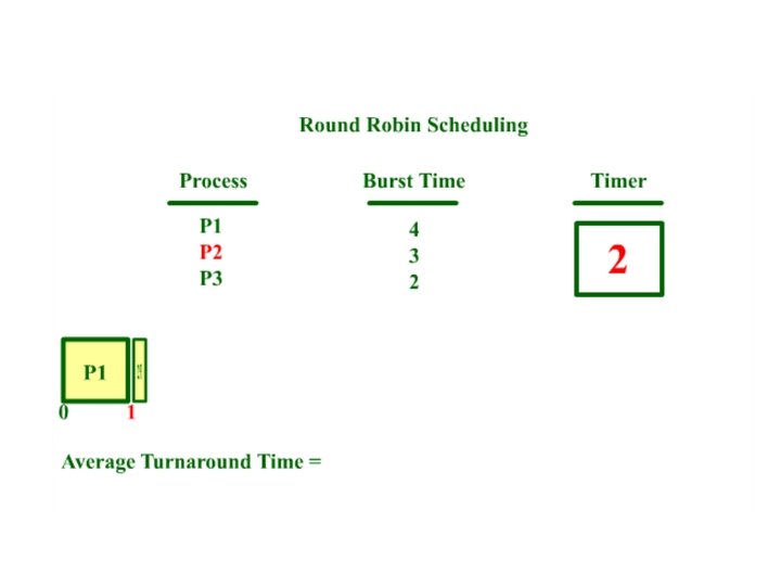
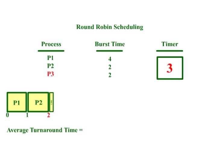
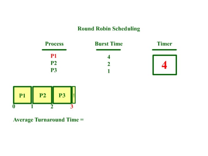
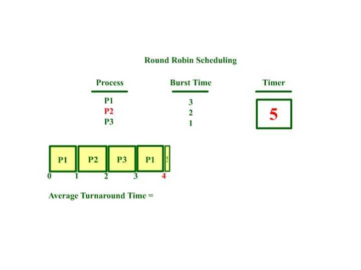
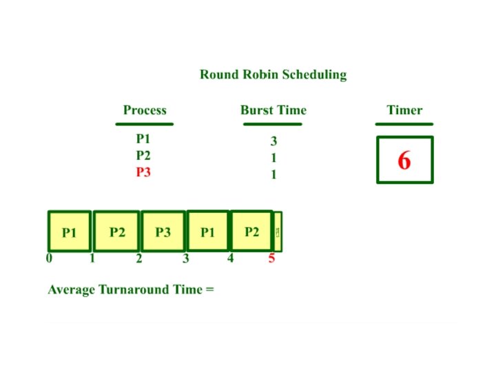
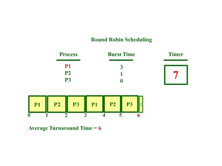
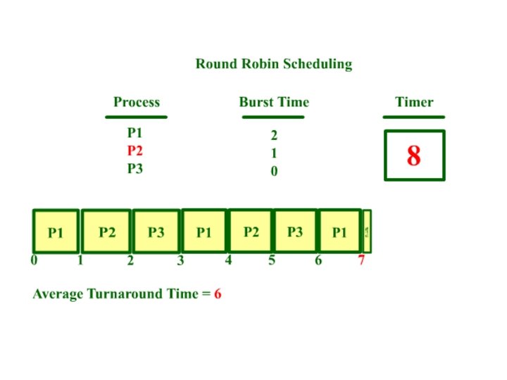
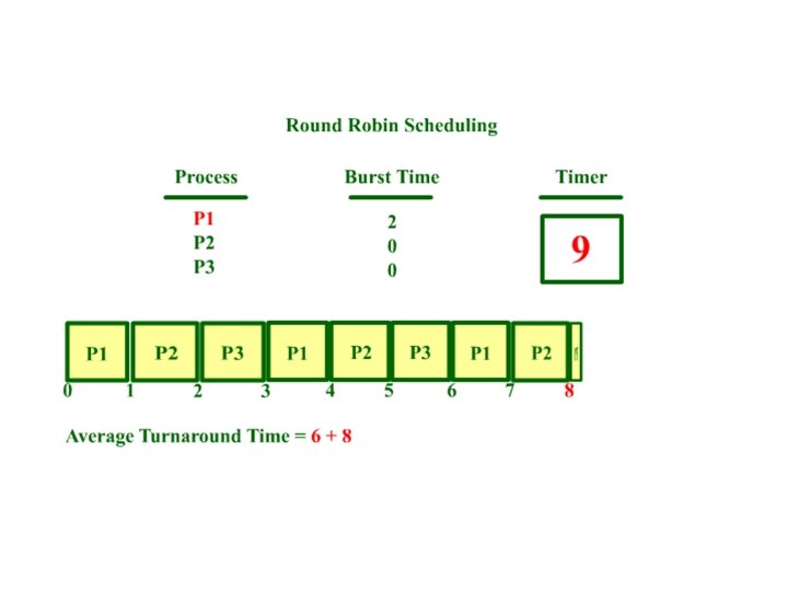
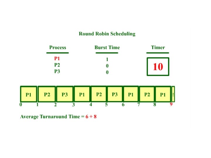
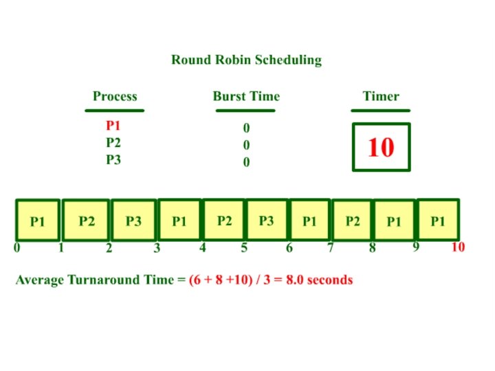
Round Robin Scheduling • Designed for time sharing systems • Preemption added to FCFS is Round Robin Scheduling • Ready queue is circular queue

Process Burst time P 1 5 P 2 3 P 3 2 WT for P 1=((3 -1)+(6 -4)+(8 -7)=5 WT for P 2=((1 -0)+((4 -2)+(7 -5)=5 WT for P 3=(2 -0)+(5 -3)=4 Avg. WT=4. 67 ATAT=8. 01 ET for P 1=5 ET for P 2=3 ET for P 3=2 Avg ET=3. 34

Comparision with FCFS • Compute the same problem using FCFS and comment on the average turnaround time • Reason out the change

Reasoning of RR • RR is heavily depended on time quantum • Lesser the time quantum, more the context switches • Turnaround time also depends on the size of the time quantum. • If time quantum is large enough then RR degenerates to FCFS • Thumb rule : 80% of cpu bursts should be shorter than the time quantum.

Process BT Priority P 1 10 3 P 2 1 1 P 3 2 3 P 4 1 4 P 5 5 2 1. 2. 3. 4. The processes are assumed to have arrived in the order P 1, p 2, p 3, p 4, p 5 Draw Gantt chart for FCFS, SJF, nonpremptive priority, RR(Time slice=1) TT of each process the above scheduling algos WT of each process for the above scheduling algos Which algo has minimum average waiting time

Multilevel queue scheduling • Based on foreground(interactive) processes and background (batch) processes multilevel queue scheduling partitions ready queues into several queues. • Each queue has its own scheduling algorithm. • scheduling among the queues, implemented as fixed-priority preemptive scheduling.

Example of multilevel queue scheduling

Multilevel Feedback Queue Scheduling • Allows a process to move between queues. • Uses the concept of aging to prevent starvation

Parameters of multilevel queue • The number of queues • The scheduling algorithm for each queue • The method used to determine when to upgrade a process to a higher priority queue • The method used to determine when to demote a process to a lower priority queue • The method used to determine which queue a process will enter when that process needs service

Operating System Examples • LINUX • Windows • Solaris

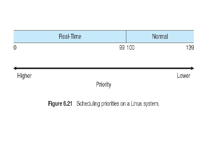
LINUX

Windows Scheduling • Uses priority-based preemptive scheduling • 32 -level priority scheme is used for scheduling • Variable class has priority from 1 to 15 and real time class has priority 16 to 31 • Windows API has 6 priority classes – – – IDLE PRIORITY CLASS BELOW NORMAL PRIORITY CLASS ABOVE NORMAL PRIORITY CLASS HIGH PRIORITY CLASS REALTIME PRIORITY CLASS

Solaris Scheduling • Uses priority based thread scheduling • Each thread belongs to one of six classes: Time sharing (TS) (default) Interactive (IA) Real time (RT) System (SYS) Fair share (FSS) Fixed priority (FP)

Solaris Scheduling Contd… • dynamically alters priorities and assigns time slices of different lengths using a multilevel feedback queue • The higher the priority, the smaller the time slice; and the lower the priority, the larger the time slice. • Interactive processes have a higher priority; CPU-bound processes, a lower priority.

RECAP • Types of schedulers • Types of scheduling algos • Examples of schedulers in different os