Cpt S 440 540 Artificial Intelligence Search Search


 state = Update. State(state, percept) if sequence is")


")


 • Queueing. Fn is Sort. By. Cost. So. Far •")

 T(1) O(3) E(2) P(5)")
 B(2) E(2) O(3) P(5)")
 E(2) O(3) P(5)")
 O(3) P(5)")
 O(3) A(3) S(5) P(5) R(6)")
 A(3) S(5) P(5) R(6)")
 A(3) S(5) P(5) R(6) G(10)")
 S(5) P(5) R(6) G(10)")
 I(4) S(5) N(5) P(5) R(6) G(10)")
 P(5) S(5) N(5) R(6) G(10)")
 S(5) N(5) R(6) Z(6) G(10)")
 N(5) R(6) Z(6) F(6) D(8) G(10) L(10)")
 R(6) Z(6) F(6) D(8) G(10) L(10)")
 F(6) D(8) G(10) L(10)")
 D(8) G(10) L(10)")


")


 • Queueing. Fn is sort-by-h – Only keep lowest-h state")


 n nodes")


 = g(n) + h(n) • Note")

 3 B (6) 15 E (20) C (20) 6 F(0) •")


 is admissible • Space is O(bm) • Features –")


 >= h 1(n) for all n")
 =")
 problem – Relaxed problem has")


 • “Like climbing Mount Everest in thick fog with amnesia”")


 // returns solution state current = Make. Node(Initial-State(problem)) for")
? – An adaptation procedure based")
 46")

 2. Do (once for")

 – Like beam")


 = #digits that match")
 0 1 1 D) 1")


- Slides: 182
Cpt. S 440 / 540 Artificial Intelligence Search
Search • Search permeates all of AI • What choices are we searching through? – Problem solving Action combinations (move 1, then move 3, then move 2. . . ) – Natural language Ways to map words to parts of speech – Computer vision Ways to map features to object model – Machine learning Possible concepts that fit examples seen so far – Motion planning Sequence of moves to reach goal destination • An intelligent agent is trying to find a set or sequence of actions to achieve a goal • This is a goal-based agent
Problem-solving Agent Simple. Problem. Solving. Agent(percept) state = Update. State(state, percept) if sequence is empty then goal = Formulate. Goal(state) problem = Formulate. Problem(state, g) sequence = Search(problem) action = First(sequence) sequence = Rest(sequence) Return action
Assumptions • Static or dynamic? Environment is static
Assumptions • Static or dynamic? • Fully or partially observable? Environment is fully observable
Assumptions • Static or dynamic? • Fully or partially observable? • Discrete or continuous? Environment is discrete
Assumptions • • Static or dynamic? Fully or partially observable? Discrete or continuous? Deterministic or stochastic? Environment is deterministic
Assumptions • • • Static or dynamic? Fully or partially observable? Discrete or continuous? Deterministic or stochastic? Episodic or sequential? Environment is sequential
Assumptions • • • Static or dynamic? Fully or partially observable? Discrete or continuous? Deterministic or stochastic? Episodic or sequential? Single agent or multiple agent?
Assumptions • • • Static or dynamic? Fully or partially observable? Discrete or continuous? Deterministic or stochastic? Episodic or sequential? Single agent or multiple agent?
Search Example Formulate goal: Be in Bucharest. Formulate problem: states are cities, operators drive between pairs of cities Find solution: Find a sequence of cities (e. g. , Arad, Sibiu, Fagaras, Bucharest) that leads from the current state to a state meeting the goal condition
Search Space Definitions • State – A description of a possible state of the world – Includes all features of the world that are pertinent to the problem • Initial state – Description of all pertinent aspects of the state in which the agent starts the search • Goal test – Conditions the agent is trying to meet (e. g. , have $1 M) • Goal state – Any state which meets the goal condition – Thursday, have $1 M, live in NYC – Friday, have $1 M, live in Valparaiso • Action – Function that maps (transitions) from one state to another
Search Space Definitions • Problem formulation – Describe a general problem as a search problem • Solution – Sequence of actions that transitions the world from the initial state to a goal state • Solution cost (additive) – Sum of the cost of operators – Alternative: sum of distances, number of steps, etc. • Search – Process of looking for a solution – Search algorithm takes problem as input and returns solution – We are searching through a space of possible states • Execution – Process of executing sequence of actions (solution)
Problem Formulation A search problem is defined by the 1. 2. 3. 4. Initial state (e. g. , Arad) Operators (e. g. , Arad -> Zerind, Arad -> Sibiu, etc. ) Goal test (e. g. , at Bucharest) Solution cost (e. g. , path cost)
Example Problems – Eight Puzzle States: tile locations Initial state: one specific tile configuration Operators: move blank tile left, right, up, or down Goal: tiles are numbered from one to eight around the square Path cost: cost of 1 per move (solution cost same as number of most or path length) Eight puzzle applet
Example Problems – Robot Assembly States: real-valued coordinates of • robot joint angles • parts of the object to be assembled Operators: rotation of joint angles Goal test: complete assembly Path cost: time to complete assembly
Example Problems – Towers of Hanoi States: combinations of poles and disks Operators: move disk x from pole y to pole z subject to constraints • cannot move disk on top of smaller disk • cannot move disk if other disks on top Goal test: disks from largest (at bottom) to smallest on goal pole Path cost: 1 per move Towers of Hanoi applet
Example Problems – Rubik’s Cube States: list of colors for each cell on each face Initial state: one specific cube configuration Operators: rotate row x or column y on face z direction a Goal: configuration has only one color on each face Path cost: 1 per move Rubik’s cube applet
Example Problems – Eight Queens States: locations of 8 queens on chess board Initial state: one specific queens configuration Operators: move queen x to row y and column z Goal: no queen can attack another (cannot be in same row, column, or diagonal) Path cost: 0 per move Eight queens applet
Example Problems – Missionaries and Cannibals States: number of missionaries, cannibals, and boat on near river bank Initial state: all objects on near river bank Operators: move boat with x missionaries and y cannibals to other side of river • no more cannibals than missionaries on either river bank or in boat • boat holds at most m occupants Goal: all objects on far river bank Path cost: 1 per river crossing Missionaries and cannibals applet
Example Problems –Water Jug States: Contents of 4 -gallon jug and 3 -gallon jug Initial state: (0, 0) Operators: • fill jug x from faucet • pour contents of jug x in jug y until y full • dump contents of jug x down drain Goal: (2, n) Path cost: 1 per fill Saving the world, Part II
Sample Search Problems • • • Graph coloring Protein folding Game playing Airline travel Proving algebraic equalities Robot motion planning
Visualize Search Space as a Tree • States are nodes • Actions are edges • Initial state is root • Solution is path from root to goal node • Edges sometimes have associated costs • States resulting from operator are children
Search Problem Example (as a tree)
Search Function – Uninformed Searches Open = initial state // open list is all generated states // that have not been “expanded” While open not empty // one iteration of search algorithm state = First(open) // current state is first state in open Pop(open) // remove new current state from open if Goal(state) // test current state for goal condition return “succeed” // search is complete // else expand the current state by // generating children and // reorder open list per search strategy else open = Queue. Function(open, Expand(state)) Return “fail”
Search Strategies • Search strategies differ only in Queuing. Function • Features by which to compare search strategies – Completeness (always find solution) – Cost of search (time and space) – Cost of solution, optimal solution – Make use of knowledge of the domain • “uninformed search” vs. “informed search”
Breadth-First Search • Generate children of a state, Queueing. Fn adds the children to the end of the open list • Level-by-level search • Order in which children are inserted on open list is arbitrary • In tree, assume children are considered left -to-right unless specified differently • Number of children is “branching factor” b
BFS Examples b=2 Example trees Search algorithms applet
Analysis • Assume goal node at level d with constant branching factor b • Time complexity (measured in #nodes generated) Ø 1 (1 st level ) + b (2 nd level) + b 2 (3 rd level) + … + bd (goal level) + (bd+1 – b) = O(bd+1) • This assumes goal on far right of level • Space complexity Ø At most majority of nodes at level d + majority of nodes at level d+1 = O(bd+1) Ø Exponential time and space • Features Ø Simple to implement Ø Complete Ø Finds shortest solution (not necessarily least-cost unless all operators have equal cost)
Analysis • See what happens with b=10 – expand 10, 000 nodes/second – 1, 000 bytes/node Depth Nodes Time Memory 2 1110 . 11 seconds 1 megabyte 4 111, 100 11 seconds 106 megabytes 6 107 19 minutes 10 gigabytes 8 109 31 hours 1 terabyte 10 1011 129 days 101 terabytes 12 1013 35 years 10 petabytes 15 1015 3, 523 years 1 exabyte
Depth-First Search • Queueing. Fn adds the children to the front of the open list • BFS emulates FIFO queue • DFS emulates LIFO stack • Net effect – Follow leftmost path to bottom, then backtrack – Expand deepest node first
DFS Examples Example trees
Analysis • Time complexity Ø Ø In the worst case, search entire space Goal may be at level d but tree may continue to level m, m>=d O(bm) Particularly bad if tree is infinitely deep • Space complexity Ø Only need to save one set of children at each level Ø 1 + b + … + b (m levels total) = O(bm) Ø For previous example, DFS requires 118 kb instead of 10 petabytes for d=12 (10 billion times less) • Benefits Ø Ø Ø May not always find solution Solution is not necessarily shortest or least cost If many solutions, may find one quickly (quickly moves to depth d) Simple to implement Space often bigger constraint, so more usable than BFS for large problems
Comparison of Search Techniques DFS BFS Complete N Y Optimal N N Heuristic N N Time bm bd+1 Space bm bd+1
Avoiding Repeated States Can we do it? • Do not return to parent or grandparent state – In 8 puzzle, do not move up right after down • Do not create solution paths with cycles • Do not generate repeated states (need to store and check potentially large number of states)
Maze Example • States are cells in a maze • Move N, E, S, or W • What would BFS do (expand E, then N, W, S)? • What would DFS do? • What if order changed to N, E, S, W and loops are prevented?
Uniform Cost Search (Branch&Bound) • Queueing. Fn is Sort. By. Cost. So. Far • Cost from root to current node n is g(n) – Add operator costs along path • First goal found is least-cost solution • Space & time can be exponential because large subtrees with inexpensive steps may be explored before useful paths with costly steps • If costs are equal, time and space are O(bd) – Otherwise, complexity related to cost of optimal solution
UCS Example Open list: C
UCS Example Open list: B(2) T(1) O(3) E(2) P(5)
UCS Example Open list: T(1) B(2) E(2) O(3) P(5)
UCS Example Open list: B(2) E(2) O(3) P(5)
UCS Example Open list: E(2) O(3) P(5)
UCS Example Open list: E(2) O(3) A(3) S(5) P(5) R(6)
UCS Example Open list: O(3) A(3) S(5) P(5) R(6)
UCS Example Open list: O(3) A(3) S(5) P(5) R(6) G(10)
UCS Example Open list: A(3) S(5) P(5) R(6) G(10)
UCS Example Open list: A(3) I(4) S(5) N(5) P(5) R(6) G(10)
UCS Example Open list: I(4) P(5) S(5) N(5) R(6) G(10)
UCS Example Open list: P(5) S(5) N(5) R(6) Z(6) G(10)
UCS Example Open list: S(5) N(5) R(6) Z(6) F(6) D(8) G(10) L(10)
UCS Example Open list: N(5) R(6) Z(6) F(6) D(8) G(10) L(10)
UCS Example Open list: Z(6) F(6) D(8) G(10) L(10)
UCS Example Open list: F(6) D(8) G(10) L(10)
UCS Example
Comparison of Search Techniques DFS BFS UCS Complete N Y Y Optimal N N Y Heuristic N N N Time bm bd+1 bm Space bm bd+1 bm
Iterative Deepening Search • DFS with depth bound • Queuing. Fn is enqueue at front as with DFS – Expand(state) only returns children such that depth(child) <= threshold – This prevents search from going down infinite path • First threshold is 1 – If do not find solution, increment threshold and repeat
Examples
Analysis • What about the repeated work? • Time complexity (number of generated nodes) Ø[b] + [b + b 2] +. . + [b + b 2 +. . + bd] Ø(d)b + (d-1) b 2 + … + (1) bd ØO(bd)
Analysis • Repeated work is approximately 1/b of total work ØNegligible ØExample: b=10, d=5 ØN(BFS) = 1, 111, 100 ØN(IDS) = 123, 450 • Features – Shortest solution, not necessarily least cost – Is there a better way to decide threshold? (IDA*)
Comparison of Search Techniques DFS BFS UCS IDS Complete N Y Y Y Optimal N N Y N Heuristic N N Time bm bd+1 bm bd Space bm bd+1 bm bd
Bidirectional Search • Search forward from initial state to goal AND backward from goal state to initial state • Can prune many options • Considerations – Which goal state(s) to use – How determine when searches overlap – Which search to use for each direction – Here, two BFS searches • Time and space is O(bd/2)
Informed Searches • Best-first search, Hill climbing, Beam search, A*, IDA*, RBFS, SMA* • New terms – – – Heuristics Optimal solution Informedness Hill climbing problems Admissibility • New parameters – g(n) = estimated cost from initial state to state n – h(n) = estimated cost (distance) from state n to closest goal – h(n) is our heuristic • Robot path planning, h(n) could be Euclidean distance • 8 puzzle, h(n) could be #tiles out of place • Search algorithms which use h(n) to guide search are heuristic search algorithms
Best-First Search • Queueing. Fn is sort-by-h • Best-first search only as good as heuristic – Example heuristic for 8 puzzle: Manhattan Distance
Example
Example
Example
Example
Example
Example
Example
Example
Example
Comparison of Search Techniques DFS BFS UCS IDS Best Complete N Y Y Y N Optimal N N Y N N Heuristic N N Y Time bm bd+1 bm bd bm Space bm bd+1 bm bd bm
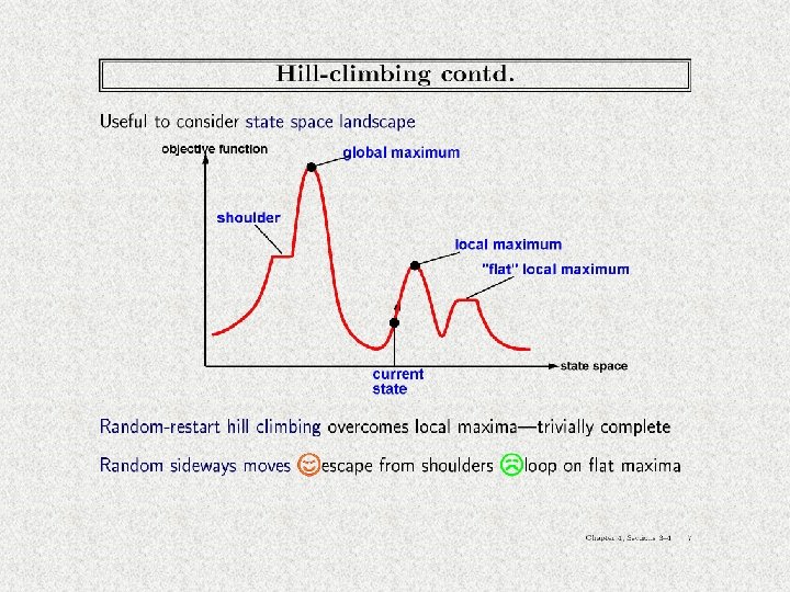
Hill Climbing (Greedy Search) • Queueing. Fn is sort-by-h – Only keep lowest-h state on open list • Best-first search is tentative • Hill climbing is irrevocable • Features – Much faster – Less memory – Dependent upon h(n) – If bad h(n), may prune away all goals – Not complete
Example
Example
Hill Climbing Issues Also referred to as gradient descent Foothill problem / local maxima / local minima Can be solved with random walk or more steps Other problems: ridges, plateaus global maxima values • • local maxima states
Comparison of Search Techniques DFS BFS UCS IDS Best HC Complete N Y Y Y N N Optimal N N Y N N N Heuristic N N Y Y Time bm bd+1 bm bd bm mn Space bm bd+1 bm bd bm b
Beam Search • Queueing. Fn is sort-by-h – Only keep best (lowest-h) n nodes on open list • n is the “beam width” – n = 1, Hill climbing – n = infinity, Best first search
Example
Example
Example
Example
Example
Example
Example
Example
Example
Comparison of Search Techniques DFS BFS UCS IDS Best HC Beam Complete N Y Y Y N N N Optimal N N Y N N Heuristic N N Y Y Y Time bm bd+1 bm bd bm bm nm Space bm bd+1 bm bd bm b bn
A* • Queueing. Fn is sort-by-f – f(n) = g(n) + h(n) • Note that UCS and Best-first both improve search – UCS keeps solution cost low – Best-first helps find solution quickly • A* combines these approaches
Power of f • If heuristic function is wrong it either – overestimates (guesses too high) – underestimates (guesses too low) • Overestimating is worse than underestimating • A* returns optimal solution if h(n) is admissible – heuristic function is admissible if never overestimates true cost to nearest goal – if search finds optimal solution using admissible heuristic, the search is admissible
Overestimating A (15) 3 B (6) 15 E (20) C (20) 6 F(0) • Solution cost: – ABF = 9 – ADI = 8 2 20 G (12) 3 D (10) 10 H (20) 5 I(0) • Open list: – A (15) B (9) F (9) • Missed optimal solution
Example A* applied to 8 puzzle A* search applet
Example
Example
Example
Example
Example
Example
Example
Example
Optimality of A* • Suppose a suboptimal goal G 2 is on the open list • Let n be unexpanded node on smallest-cost path to optimal goal G 1 f(G 2) = g(G 2) since h(G 2) = 0 >= g(G 1) since G 2 is suboptimal >= f(n) since h is admissible Since f(G 2) > f(n), A* will never select G 2 for expansion
Comparison of Search Techniques DFS BFS UCS IDS Best HC Beam A* Complete N Y Y Y N N N Y Optimal N N Y Heuristic N N Y Y Time bm bd+1 bm bd bm bm nm bm Space bm bd+1 bm bd bm b bn bm
IDA* • Series of Depth-First Searches • Like Iterative Deepening Search, except – Use A* cost threshold instead of depth threshold – Ensures optimal solution • Queuing. Fn enqueues at front if f(child) <= threshold • Threshold – h(root) first iteration – Subsequent iterations • f(min_child) • min_child is the cut off child with the minimum f value – Increase always includes at least one new node – Makes sure search never looks beyond optimal cost solution
Example
Example
Example
Example
Example
Example
Example
Example
Example
Example
Example
Example
Example
Example
Example
Example
Example
Example
Example
Example
Example
Example
Example
Example
Example
Example
Example
Example
Analysis • Some redundant search – Small amount compared to work done on last iteration • Dangerous if continuous-valued h(n) values or if values very close – If threshold = 21. 1 and value is 21. 2, probably only include 1 new node each iteration • Time complexity is O(bm) • Space complexity is O(m)
Comparison of Search Techniques DFS BFS UCS IDS Best HC Beam A* IDA* Complete N Y Y Y N N N Y Y Optimal N N Y Y Heuristic N N Y Y Y Time bm bd+1 bm bd bm bm nm bm bm Space bm bd+1 bm bd bm b bn bm bm
RBFS • Recursive Best First Search – Linear space variant of A* • Perform A* search but discard subtrees when perform recursion • Keep track of alternative (next best) subtree • Expand subtree until f value greater than bound • Update f values before (from parent) and after (from descendant) recursive call
Algorithm // Input is current node and f limit // Returns goal node or failure, updated limit RBFS(n, limit) if Goal(n) return n children = Expand(n) if children empty return failure, infinity for each c in children f[c] = max(g(c)+h(c), f[n]) // Update f[c] based on parent repeat best = child with smallest f value if f[best] > limit return failure, f[best] alternative = second-lowest f-value among children newlimit = min(limit, alternative) result, f[best] = RBFS(best, newlimit) // Update f[best] based on descendant if result not equal to failure return result
Example
Example
Example
Example
Example
Example
Analysis • Optimal if h(n) is admissible • Space is O(bm) • Features – Potentially exponential time in cost of solution – More efficient than IDA* – Keeps more information than IDA* but benefits from storing this information
SMA* • Simplified Memory-Bounded A* Search • Perform A* search • When memory is full – Discard worst leaf (largest f(n) value) – Back value of discarded node to parent • Optimal if solution fits in memory
Example • Let Max. Nodes = 3 • Initially B&G added to open list, then hit max • B is larger f value so discard but save f(B)=15 at parent A – Add H but f(H)=18. Not a goal and cannot go deper, so set f(h)=infinity and save at G. • Generate next child I with f(I)=24, bigger child of A. We have seen all children of G, so reset f(G)=24. • Regenerate B and child C. This is not goal so f(c) reset to infinity • Generate second child D with f(D)=24, backing up value to ancestors • D is a goal node, so search terminates.
Heuristic Functions • Q: Given that we will only use heuristic functions that do not overestimate, what type of heuristic functions (among these) perform best? • A: Those that produce higher h(n) values.
Reasons • Higher h value means closer to actual distance • Any node n on open list with – f(n) < f*(goal) – will be selected for expansion by A* • This means if a lot of nodes have a low underestimate (lower than actual optimum cost) – All of them will be expanded – Results in increased search time and space
Informedness • If h 1 and h 2 are both admissible and • For all x, h 1(x) > h 2(x), then h 1 “dominates” h 2 – Can also say h 1 is “more informed” than h 2 • Example – h 1(x): – h 2(x): Euclidean distance – h 2 dominates h 1
Effect on Search Cost • If h 2(n) >= h 1(n) for all n (both are admissible) – then h 2 dominates h 1 and is better for search • Typical search costs – d=14, IDS expands 3, 473, 941 nodes • A* with h 1 expands 539 nodes • A* with h 2 expands 113 nodes – d=24, IDS expands ~54, 000, 000 nodes • A* with h 1 expands 39, 135 nodes • A* with h 2 expands 1, 641 nodes
Which of these heuristics are admissible? Which are more informed? • h 1(n) = #tiles in wrong position • h 2(n) = Sum of Manhattan distance between each tile and goal location for the tile • h 3(n) = 0 • h 4(n) = 1 • h 5(n) = min(2, h*[n]) • h 6(n) = Manhattan distance for blank tile • h 7(n) = max(2, h*[n])
Generating Heuristic Functions • Generate heuristic for simpler (relaxed) problem – Relaxed problem has fewer restrictions – Eight puzzle where multiple tiles can be in the same spot – Cost of optimal solution to relaxed problem is an admissible heuristic for the original problem • Learn heuristic from experience
Iterative Improvement Algorithms • Hill climbing • Simulated annealing • Genetic algorithms
Iterative Improvement Algorithms • For many optimization problems, solution path is irrelevant – Just want to reach goal state • State space / search space – Set of “complete” configurations – Want to find optimal configuration (or at least one that satisfies goal constraints) • For these cases, use iterative improvement algorithm – Keep a single current state – Try to improve it • Constant memory
Example • Traveling salesman • Start with any complete tour • Operator: Perform pairwise exchanges
Example • N-queens • Put n queens on an n × n board with no two queens on the same row, column, or diagonal • Operator: Move queen to reduce #conflicts
Hill Climbing (gradient ascent/descent) • “Like climbing Mount Everest in thick fog with amnesia”
Local Beam Search • Keep k states instead of 1 • Choose top k of all successors • Problem – Many times all k states end up on same local hill – Choose k successors RANDOMLY – Bias toward good ones • Similar to natural selection
Simulated Annealing • Pure hill climbing is not complete, but pure random search is inefficient. • Simulated annealing offers a compromise. • Inspired by annealing process of gradually cooling a liquid until it changes to a low-energy state. • Very similar to hill climbing, except include a user-defined temperature schedule. • When temperature is “high”, allow some random moves. • When temperature “cools”, reduce probability of random move. • If T is decreased slowly enough, guaranteed to reach best state.
Algorithm function Simulated. Annealing(problem, schedule) // returns solution state current = Make. Node(Initial-State(problem)) for t = 1 to infinity T = schedule[t] if T = 0 return current next = randomly-selected child of current = Value[next] - Value[current] if >0 current = next // if better than accept state else current = next with probability Simulated annealing applet Traveling salesman simulated annealing applet
Genetic Algorithms • What is a Genetic Algorithm (GA)? – An adaptation procedure based on the mechanics of natural genetics and natural selection • Gas have 2 essential components – Survival of the fittest – Recombination • Representation – Chromosome = string – Gene = single bit or single subsequence in string, represents 1 attribute
Humans • • DNA made up of 4 nucleic acids (4 -bit code) 46 chromosomes in humans, each contain 3 billion DNA 43 billion combinations of bits Can random search find humans? – – Assume only 0. 1% genome must be discovered, 3(106) nucleotides Assume very short generation, 1 generation/second 107 7) 10 1. 8(10 3. 2( 6 ) individuals per year, but 10 alternatives 10 1018 years to generate human randomly • Self reproduction, self repair, adaptability are the rule in natural systems, they hardly exist in the artificial world • Finding and adopting nature’s approach to computational design should unlock many doors in science and engineering
GAs Exhibit Search • Each attempt a GA makes towards a solution is called a chromosome – A sequence of information that can be interpreted as a possible solution • Typically, a chromosome is represented as sequence of binary digits – Each digit is a gene • A GA maintains a collection or population of chromosomes – Each chromosome in the population represents a different guess at the solution
The GA Procedure 1. Initialize a population (of solution guesses) 2. Do (once for each generation) a. Evaluate each chromosome in the population using a fitness function b. Apply GA operators to population to create a new population 3. Finish when solution is reached or number of generations has reached an allowable maximum.
Common Operators • Reproduction • Crossover • Mutation
Reproduction • Select individuals x according to their fitness values f(x) – Like beam search • Fittest individuals survive (and possibly mate) for next generation
Crossover • Select two parents • Select cross site • Cut and splice pieces of one parent to those of the other 11111 00000 11000 00111
Mutation • • With small probability, randomly alter 1 bit Minor operator An insurance policy against lost bits Pushes out of local minima Population: Goal: 0 1 1 110000 101000 10010000 Mutation needed to find the goal
Example • Solution = 0 0 1 0 • Fitness(x) = #digits that match solution A) 0 1 0 1 Score: 1 B) 1 1 0 1 Score: 1 C) 0 1 1 Score: 3 D) 1 0 1 1 0 0 Score: 3 Recombine top two twice. Note: 64 possible combinations
Example • Solution = 0 0 1 0 C) 0 1 1 D) 1 0 1 1 0 0 • Next generation: E) 0 0 1 1 0 0 F) 0 1 1 0 E) 0 | 0 1 1 0 0 F) 1 | 1 1 0 1 1 G) 0 1 1 0 1 | 0 Score: 4 H) 1 0 1 1 0 | 1 Score: 2 G) 0 1 1 | 1 0 0 Score: 3 H) 0 0 1 | 0 1 0 Score: 6 I) 0 0 | 1 0 J) 0 1 | 1 1 0 0 Score: 4 Score: 3 Score: 6 Score: 3 DONE! Got it in 10 guesses.
Issues How select original population? How handle non-binary solution types? What should be the size of the population? What is the optimal mutation rate? How are mates picked for crossover? Can any chromosome appear more than once in a population? • When should the GA halt? • Local minima? • Parallel algorithms? • • •
GAs for Mazes
GAs for Optimization • Traveling salesman problem • Eaters • Hierarchical GAs for game playing
GAs for Control • Simulator
GAs for Graphic Animation • • Simulator Evolving Circles 3 D Animation Scientific American Frontiers
Biased Roulette Wheel • For each hypothesis, spin the roulette wheel to determine the guess
Inversion • Invert selected subsequence • 1 0 | 1 1 -> 1 0 0 1 1
Elitism • Some of the best chromosomes from previous generation replace some of the worst chromosomes from current generation
K-point crossover • Pick k random splice points to crossover parents • Example – K=3 11|11|11111 00|00|00000 -> 1100000 0011111
Diversity Measure • Fitness ignores diversity • As a result, populations tend to become uniform • Rank-space method – Sort population by sum of fitness rank and diversity rank – Diversity rank is the result of sorting by the function 1/d 2
Classifier Systems • GAs and load balancing • SAMUEL