Cpr E 281 Digital Logic Instructor Alexander Stoytchev

![Let’s Draw the K-map [ Figure 2. 33 a from the textbook ] Let’s Draw the K-map [ Figure 2. 33 a from the textbook ]](https://slidetodoc.com/presentation_image_h/884c0629a2f843cc1fb25be0edc3ba75/image-8.jpg)
![Let’s Draw the K-map again [ Figure 2. 33 a from the textbook ] Let’s Draw the K-map again [ Figure 2. 33 a from the textbook ]](https://slidetodoc.com/presentation_image_h/884c0629a2f843cc1fb25be0edc3ba75/image-24.jpg)
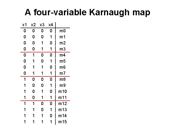
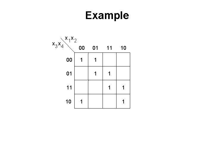
![A four-variable Karnaugh map [ Figure 2. 53 from the textbook ] A four-variable Karnaugh map [ Figure 2. 53 from the textbook ]](https://slidetodoc.com/presentation_image_h/884c0629a2f843cc1fb25be0edc3ba75/image-45.jpg)

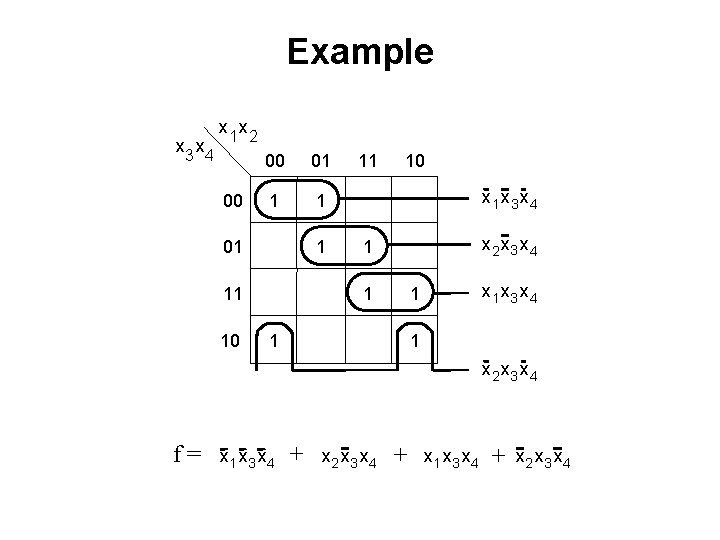
![Example of a four-variable Karnaugh map [ Figure 2. 54 from the textbook ] Example of a four-variable Karnaugh map [ Figure 2. 54 from the textbook ]](https://slidetodoc.com/presentation_image_h/884c0629a2f843cc1fb25be0edc3ba75/image-54.jpg)
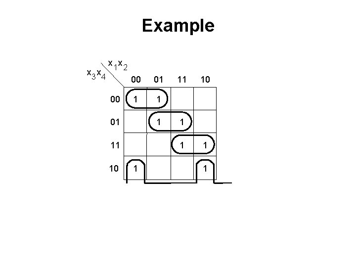
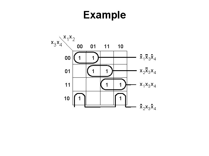
![Example of a four-variable Karnaugh map [ Figure 2. 54 from the textbook ] Example of a four-variable Karnaugh map [ Figure 2. 54 from the textbook ]](https://slidetodoc.com/presentation_image_h/884c0629a2f843cc1fb25be0edc3ba75/image-55.jpg)




- Slides: 92

Cpr. E 281: Digital Logic Instructor: Alexander Stoytchev http: //www. ece. iastate. edu/~alexs/classes/

Minimization Cpr. E 281: Digital Logic Iowa State University, Ames, IA Copyright © Alexander Stoytchev

Administrative Stuff • HW 4 is out • It is due on Monday Sep 17 @ 4 pm • It is posted on the class web page • I also sent you an e-mail with the link.

Example: K-Map for the 2 -1 Multiplexer

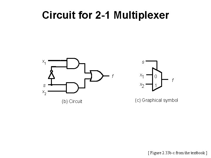
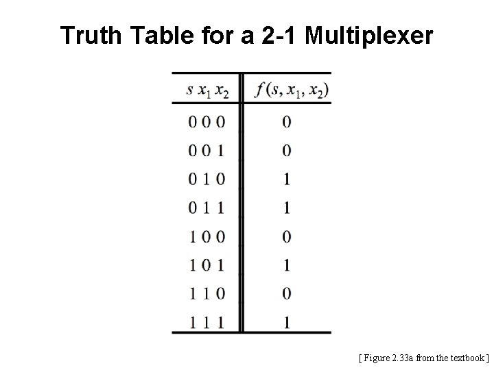
2 -1 Multiplexer (Definition) • Has two inputs: x 1 and x 2 • Also has another input line s • If s=0, then the output is equal to x 1 • If s=1, then the output is equal to x 2

Circuit for 2 -1 Multiplexer x 1 s f s x 2 (b) Circuit x 1 0 x 2 1 f (c) Graphical symbol [ Figure 2. 33 b-c from the textbook ]

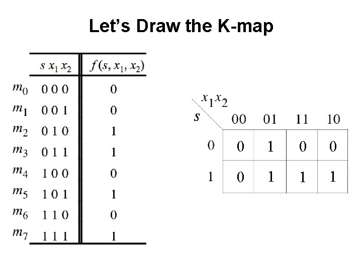
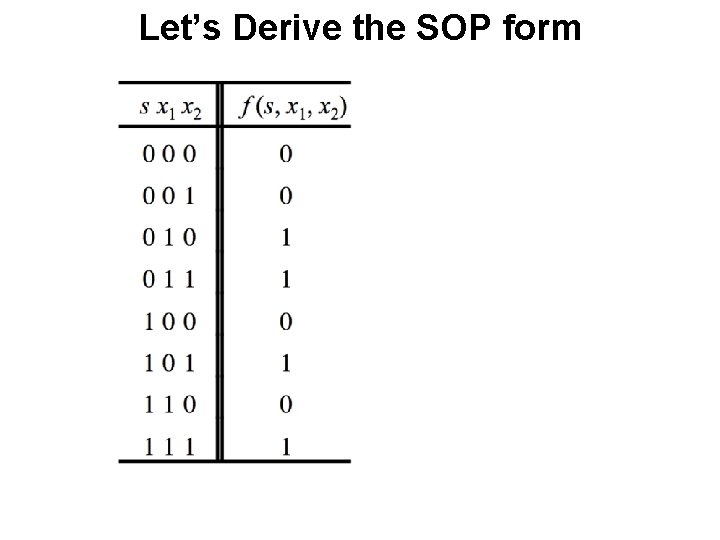
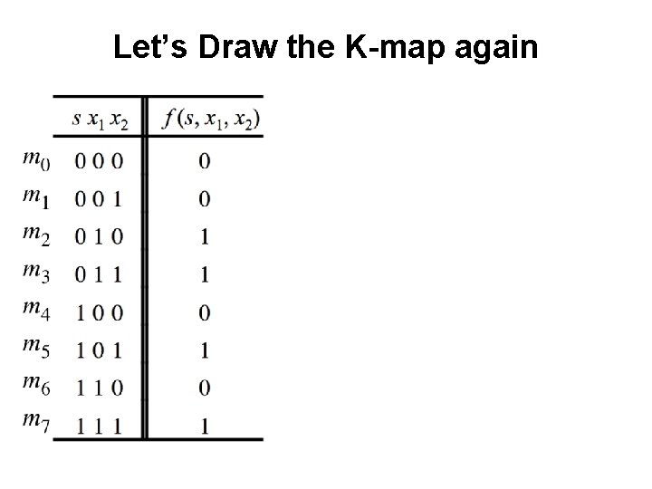
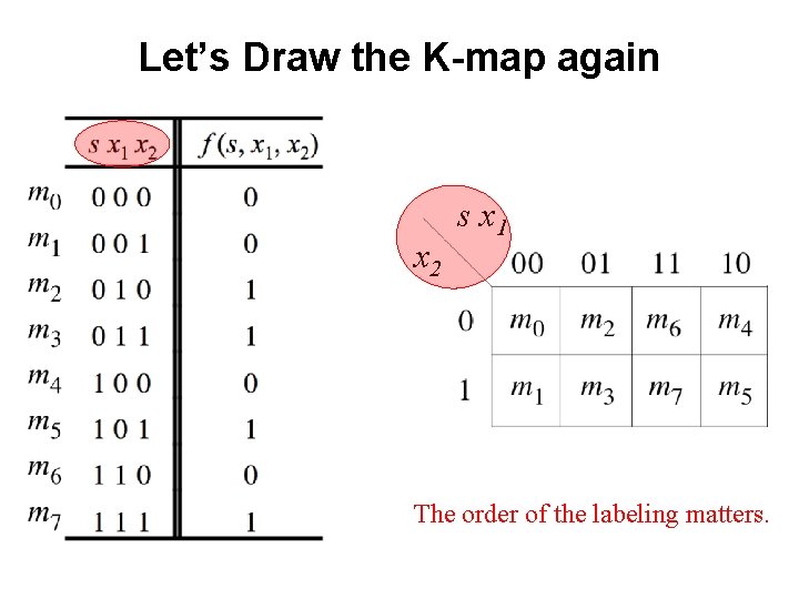
Truth Table for a 2 -1 Multiplexer [ Figure 2. 33 a from the textbook ]
![Lets Draw the Kmap Figure 2 33 a from the textbook Let’s Draw the K-map [ Figure 2. 33 a from the textbook ]](https://slidetodoc.com/presentation_image_h/884c0629a2f843cc1fb25be0edc3ba75/image-8.jpg)
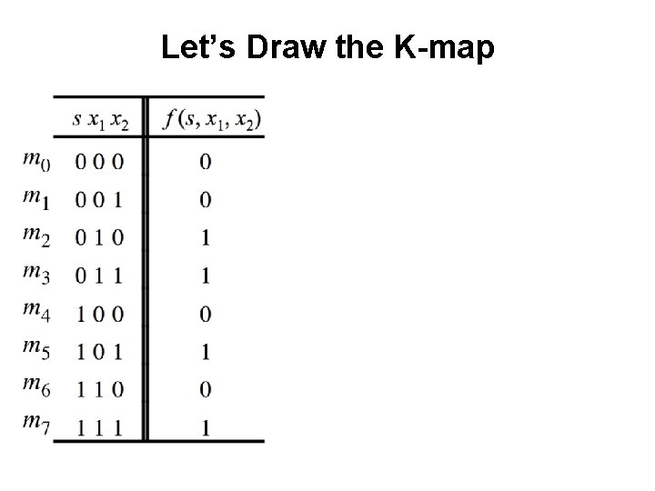
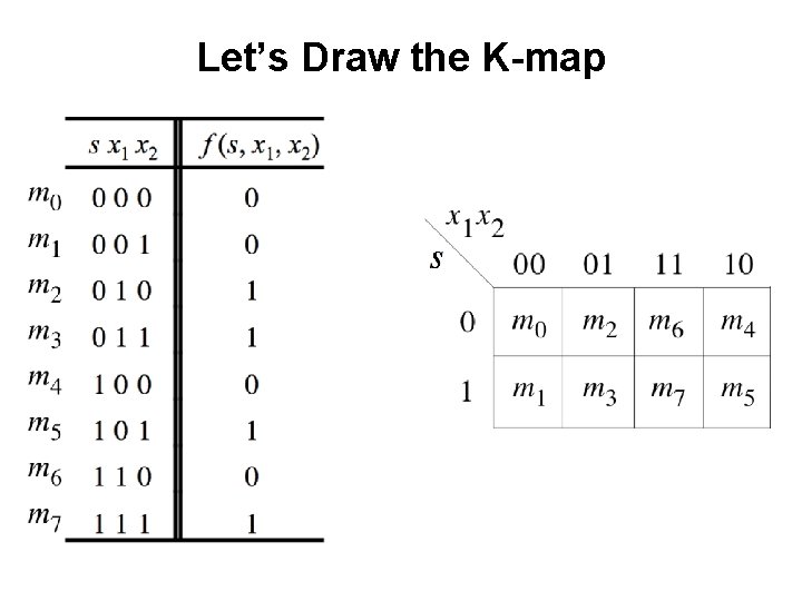
Let’s Draw the K-map [ Figure 2. 33 a from the textbook ]

Let’s Draw the K-map

Let’s Draw the K-map

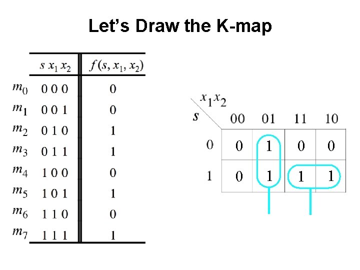
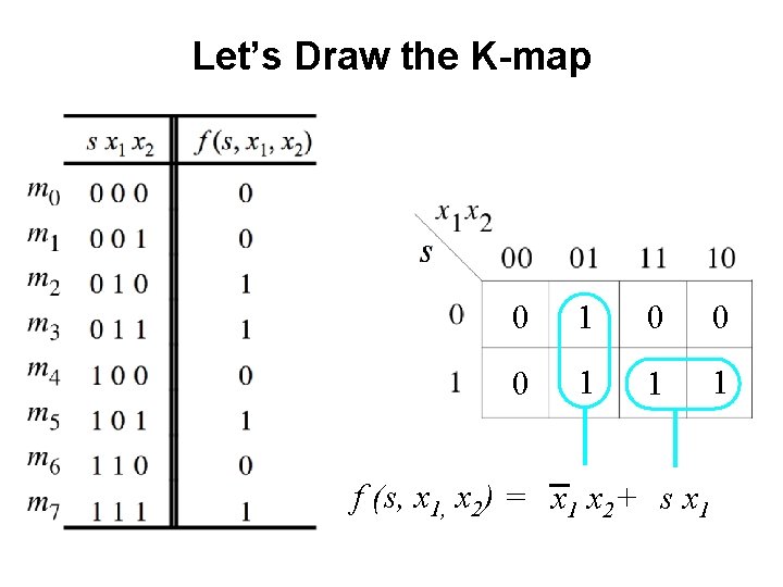
Let’s Draw the K-map 0 1 0 0 0 1 1 1

Let’s Draw the K-map 0 1 0 0 0 1 1 1

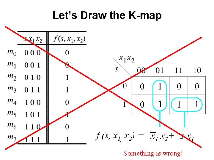
Let’s Draw the K-map 0 1 0 0 0 1 1 1 f (s, x 1, x 2) = x 1 x 2+ s x 1

Let’s Draw the K-map 0 1 0 0 0 1 1 1 f (s, x 1, x 2) = x 1 x 2+ s x 1 Something is wrong!

Compare this with the SOP derivation

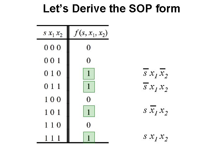
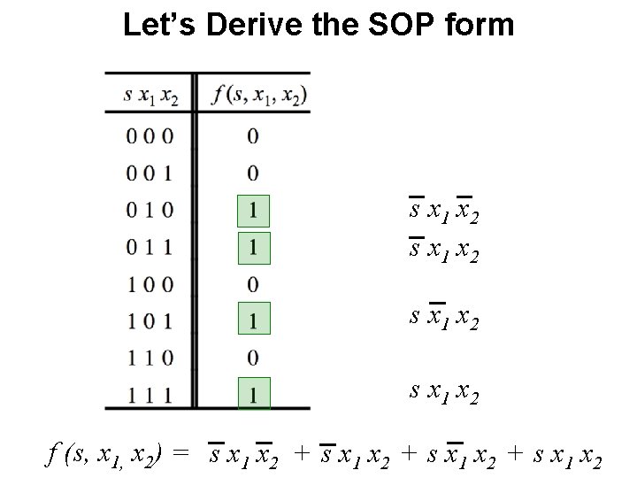
Let’s Derive the SOP form

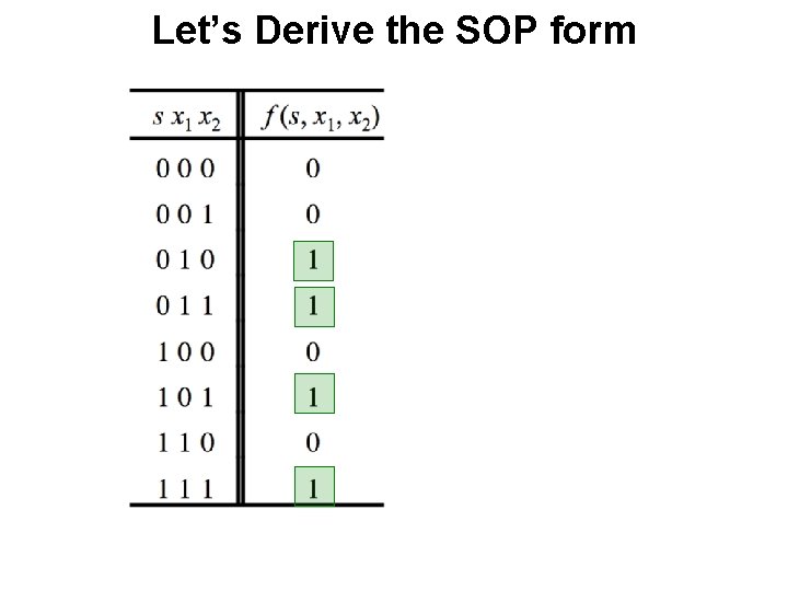
Let’s Derive the SOP form

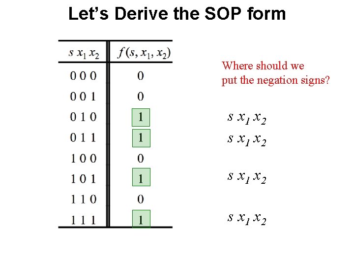
Let’s Derive the SOP form Where should we put the negation signs? s x 1 x 2

Let’s Derive the SOP form s x 1 x 2

Let’s Derive the SOP form s x 1 x 2 f (s, x 1, x 2) = s x 1 x 2 + s x 1 x 2

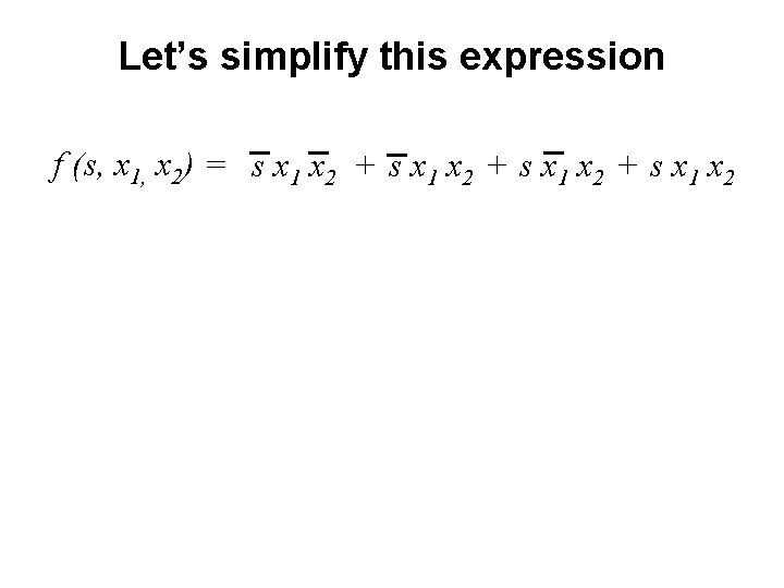
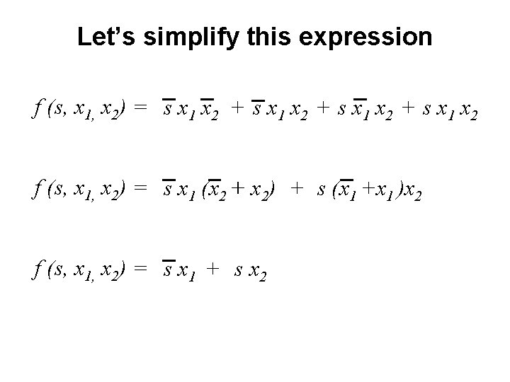
Let’s simplify this expression f (s, x 1, x 2) = s x 1 x 2 + s x 1 x 2

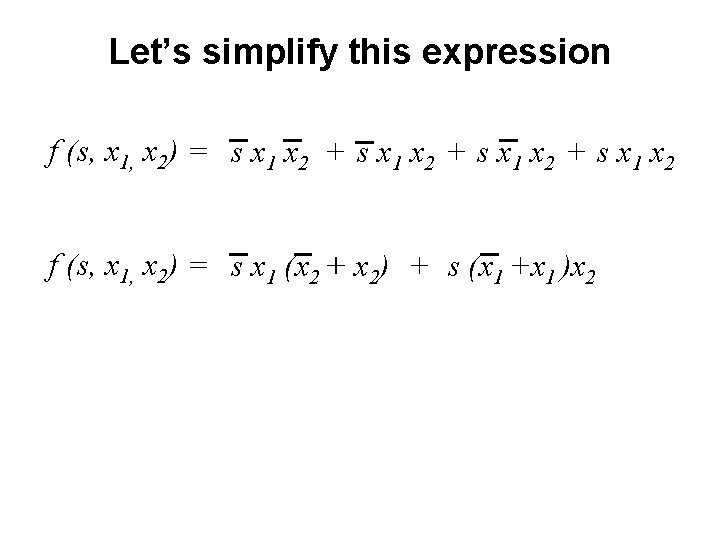
Let’s simplify this expression f (s, x 1, x 2) = s x 1 x 2 + s x 1 x 2 f (s, x 1, x 2) = s x 1 (x 2 + x 2) + s (x 1 +x 1 )x 2

Let’s simplify this expression f (s, x 1, x 2) = s x 1 x 2 + s x 1 x 2 f (s, x 1, x 2) = s x 1 (x 2 + x 2) + s (x 1 +x 1 )x 2 f (s, x 1, x 2) = s x 1 + s x 2
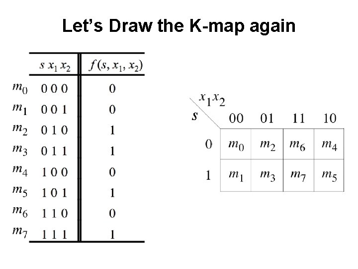
![Lets Draw the Kmap again Figure 2 33 a from the textbook Let’s Draw the K-map again [ Figure 2. 33 a from the textbook ]](https://slidetodoc.com/presentation_image_h/884c0629a2f843cc1fb25be0edc3ba75/image-24.jpg)
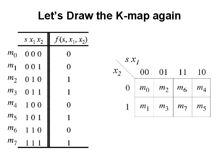
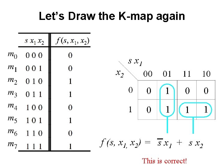
Let’s Draw the K-map again [ Figure 2. 33 a from the textbook ]

Let’s Draw the K-map again

Let’s Draw the K-map again

Let’s Draw the K-map again

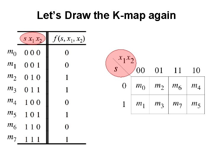
Let’s Draw the K-map again x 2 s x 1 The order of the labeling matters.

Let’s Draw the K-map again x 2 s x 1

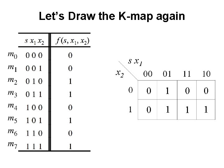
Let’s Draw the K-map again x 2 s x 1 0 0 0 1 1 1

Let’s Draw the K-map again x 2 s x 1 0 0 0 1 1 1

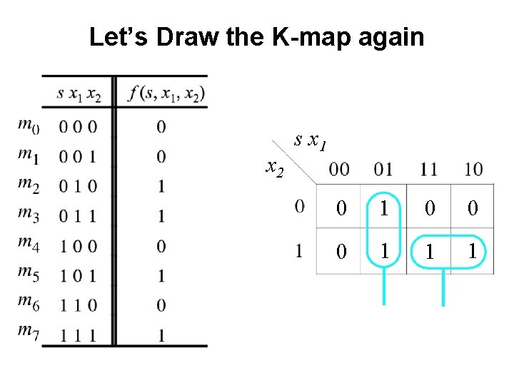
Let’s Draw the K-map again x 2 s x 1 0 0 0 1 1 1 f (s, x 1, x 2) = s x 1 + s x 2 This is correct!

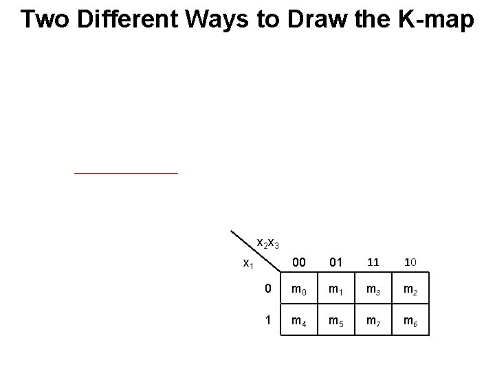
Two Different Ways to Draw the K-map x 2 x 3 00 01 11 10 0 m 1 m 3 m 2 1 m 4 m 5 m 7 m 6 x 1

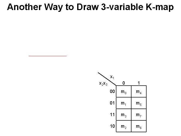
Another Way to Draw 3 -variable K-map x 1 x 2 x 3 0 1 00 m 4 01 m 5 11 m 3 m 7 10 m 2 m 6

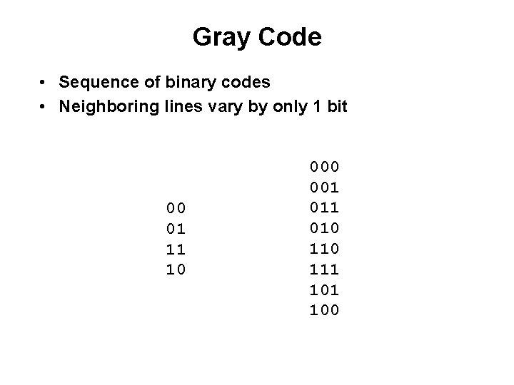
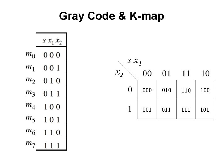
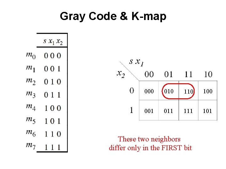
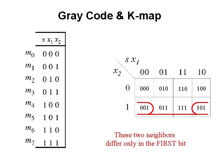
Gray Code • Sequence of binary codes • Neighboring lines vary by only 1 bit 00 01 11 10 001 010 111 100

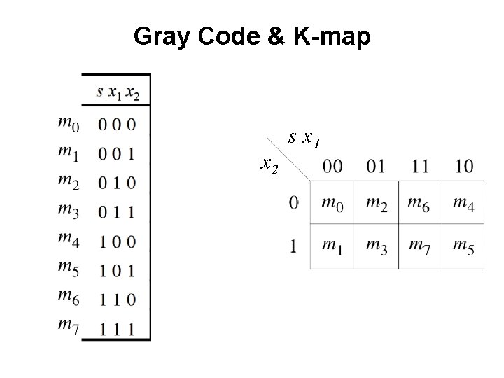
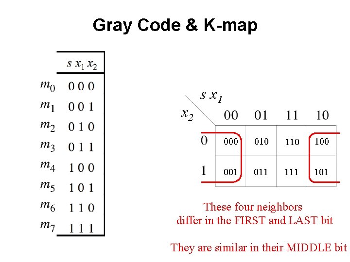
Gray Code & K-map x 2 s x 1

Gray Code & K-map x 2 s x 1 000 010 100 001 011 101

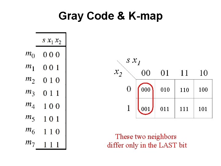
Gray Code & K-map x 2 s x 1 000 010 100 001 011 101 These two neighbors differ only in the LAST bit

Gray Code & K-map x 2 s x 1 000 010 100 001 011 101 These two neighbors differ only in the LAST bit

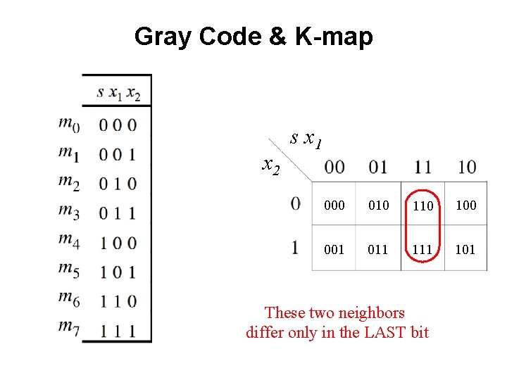
Gray Code & K-map x 2 s x 1 000 010 100 001 011 101 These two neighbors differ only in the FIRST bit

Gray Code & K-map x 2 s x 1 000 010 100 001 011 101 These two neighbors differ only in the FIRST bit

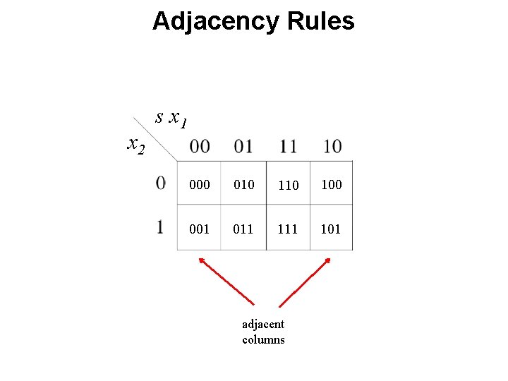
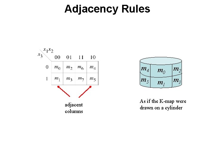
Adjacency Rules x 2 s x 1 000 010 100 001 011 101 adjacent columns

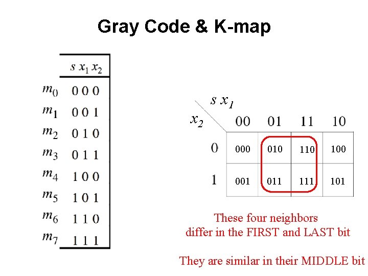
Gray Code & K-map x 2 s x 1 000 010 100 001 011 101 These four neighbors differ in the FIRST and LAST bit They are similar in their MIDDLE bit

Gray Code & K-map x 2 s x 1 000 010 100 001 011 101 These four neighbors differ in the FIRST and LAST bit They are similar in their MIDDLE bit
![A fourvariable Karnaugh map Figure 2 53 from the textbook A four-variable Karnaugh map [ Figure 2. 53 from the textbook ]](https://slidetodoc.com/presentation_image_h/884c0629a2f843cc1fb25be0edc3ba75/image-45.jpg)
A four-variable Karnaugh map [ Figure 2. 53 from the textbook ]

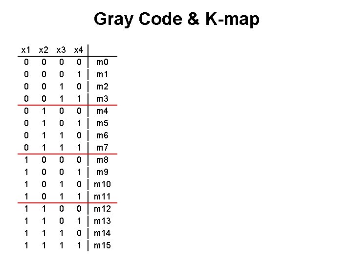
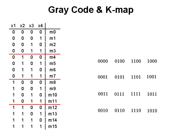
A four-variable Karnaugh map x 1 x 2 x 3 x 4 0 0 0 0 1 1 0 0 0 1 0 1 1 0 0 0 1 1 0 1 0 1 1 0 0 1 1 1 1 0 1 1 m 0 m 1 m 2 m 3 m 4 m 5 m 6 m 7 m 8 m 9 m 10 m 11 m 12 m 13 m 14 m 15

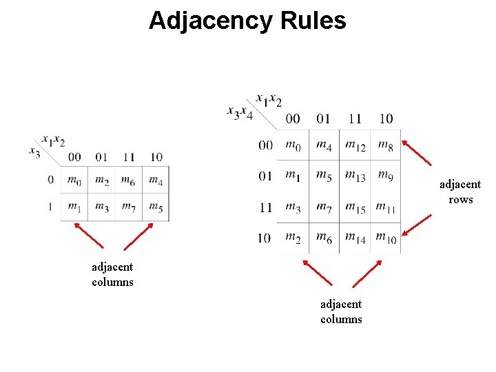
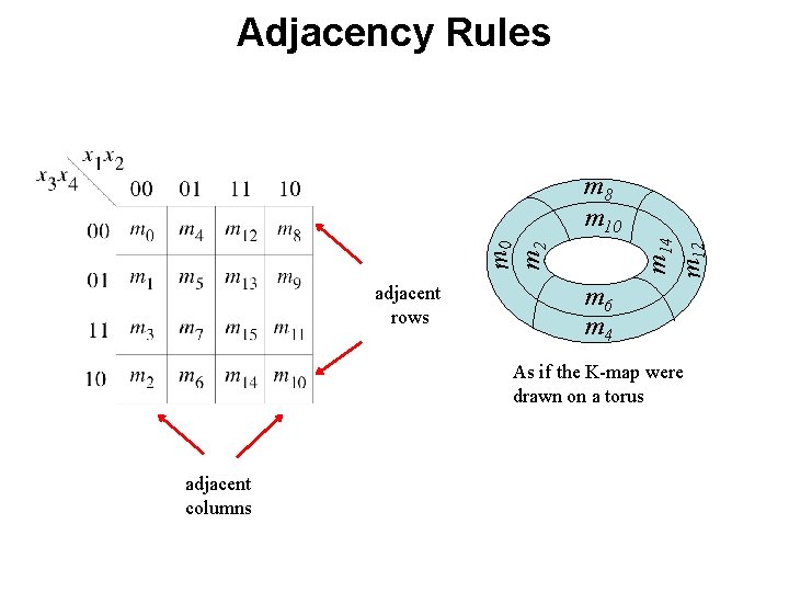
Adjacency Rules adjacent rows adjacent columns

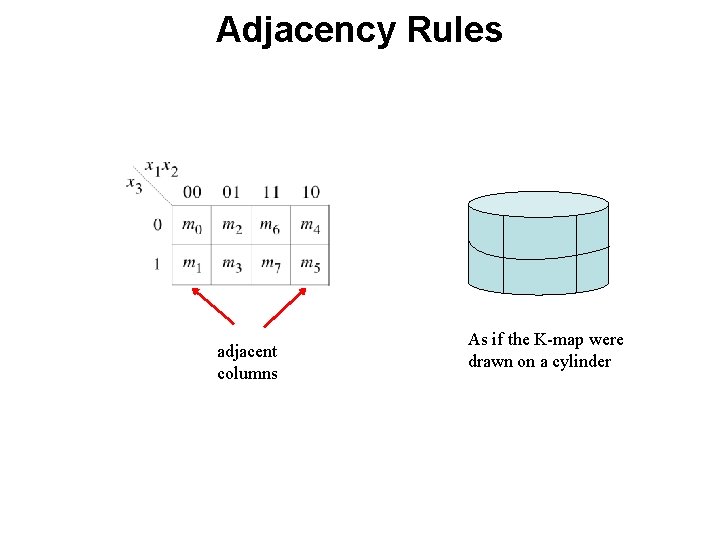
Adjacency Rules adjacent columns As if the K-map were drawn on a cylinder

Adjacency Rules adjacent columns m 4 m 0 m 2 m 5 m 1 m 3 As if the K-map were drawn on a cylinder

Adjacency Rules adjacent rows As if the K-map were drawn on a torus adjacent columns

Adjacency Rules m 0 m 2 m 14 m 12 m 8 m 10 adjacent rows m 6 m 4 As if the K-map were drawn on a torus adjacent columns

Gray Code & K-map x 1 x 2 x 3 x 4 0 0 0 0 1 1 0 0 0 1 0 1 1 0 0 0 1 1 0 1 0 1 1 0 0 1 1 1 1 0 1 1 m 0 m 1 m 2 m 3 m 4 m 5 m 6 m 7 m 8 m 9 m 10 m 11 m 12 m 13 m 14 m 15

Gray Code & K-map x 1 x 2 x 3 x 4 0 0 0 0 1 1 0 0 0 1 0 1 1 0 0 0 1 1 0 1 0 1 1 0 0 1 1 1 1 0 1 1 m 0 m 1 m 2 m 3 m 4 m 5 m 6 m 7 m 8 m 9 m 10 m 11 m 12 m 13 m 14 m 15 0000 0100 1000 0001 0101 1001 0011 0111 1011 0010 0110 1010
![Example of a fourvariable Karnaugh map Figure 2 54 from the textbook Example of a four-variable Karnaugh map [ Figure 2. 54 from the textbook ]](https://slidetodoc.com/presentation_image_h/884c0629a2f843cc1fb25be0edc3ba75/image-54.jpg)
Example of a four-variable Karnaugh map [ Figure 2. 54 from the textbook ]
![Example of a fourvariable Karnaugh map Figure 2 54 from the textbook Example of a four-variable Karnaugh map [ Figure 2. 54 from the textbook ]](https://slidetodoc.com/presentation_image_h/884c0629a2f843cc1fb25be0edc3ba75/image-55.jpg)
Example of a four-variable Karnaugh map [ Figure 2. 54 from the textbook ]

Strategy For Minimization

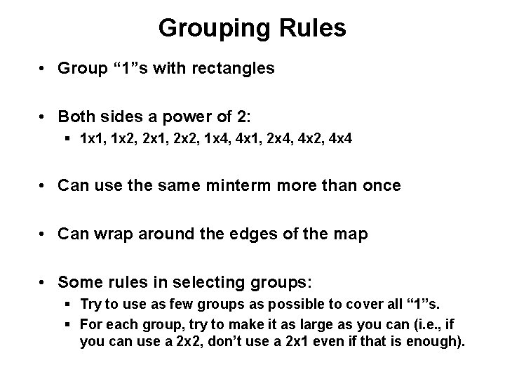
Grouping Rules • Group “ 1”s with rectangles • Both sides a power of 2: § 1 x 1, 1 x 2, 2 x 1, 2 x 2, 1 x 4, 4 x 1, 2 x 4, 4 x 2, 4 x 4 • Can use the same minterm more than once • Can wrap around the edges of the map • Some rules in selecting groups: § Try to use as few groups as possible to cover all “ 1”s. § For each group, try to make it as large as you can (i. e. , if you can use a 2 x 2, don’t use a 2 x 1 even if that is enough).

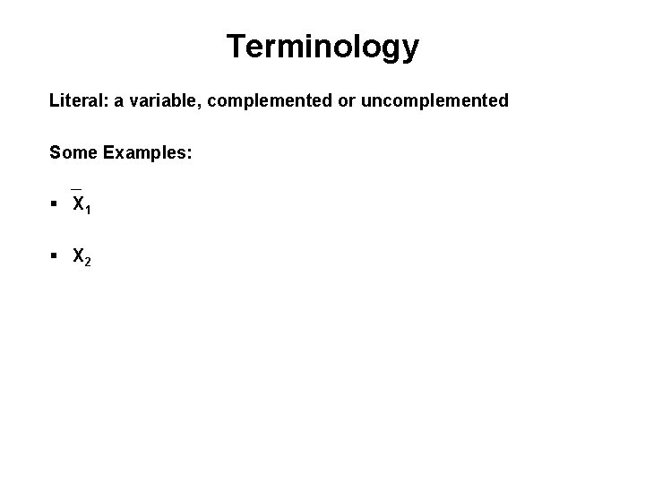
Terminology Literal: a variable, complemented or uncomplemented Some Examples: _ § X 1 § X 2

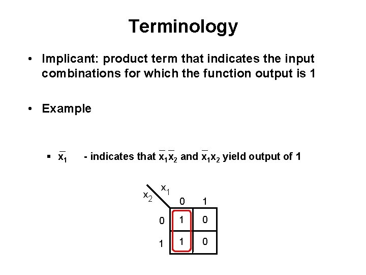
Terminology • Implicant: product term that indicates the input combinations for which the function output is 1 • Example _ § x 1 __ _ - indicates that x 1 x 2 and x 1 x 2 yield output of 1 x 2 x 1 0 1 0 1 1 0

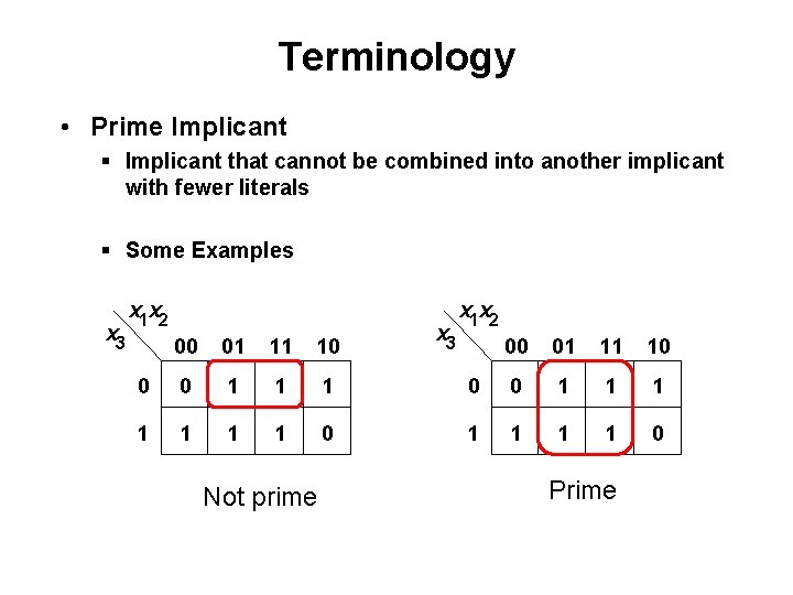
Terminology • Prime Implicant § Implicant that cannot be combined into another implicant with fewer literals § Some Examples x 3 x 1 x 2 00 01 11 10 0 0 1 1 1 1 0 Not prime x 3 x 1 x 2 00 01 11 10 0 0 1 1 1 1 0 Prime

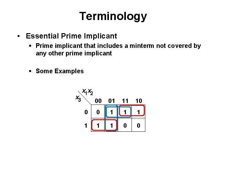
Terminology • Essential Prime Implicant § Prime implicant that includes a minterm not covered by any other prime implicant § Some Examples x 3 x 1 x 2 00 01 11 10 0 0 1 1 1 0 0

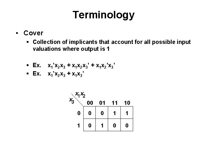
Terminology • Cover § Collection of implicants that account for all possible input valuations where output is 1 § Ex. x 1’x 2 x 3 + x 1 x 2 x 3’ + x 1 x 2’x 3’ x 1’x 2 x 3 + x 1 x 3’ x 3 x 1 x 2 00 01 11 10 0 1 1 1 0 0

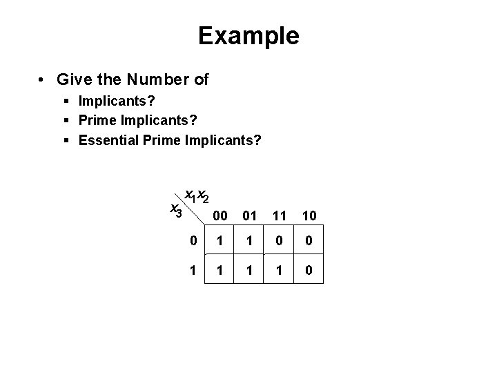
Example • Give the Number of § Implicants? § Prime Implicants? § Essential Prime Implicants? x 3 x 1 x 2 00 01 11 10 0 1 1 1 1 0

Why concerned with minimization? • Simplified function • Reduce the cost of the circuit § Cost: Gates + Inputs § Transistors

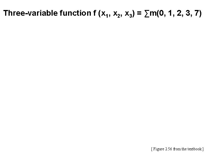
Three-variable function f (x 1, x 2, x 3) = ∑m(0, 1, 2, 3, 7) [ Figure 2. 56 from the textbook ]

Example x 3 x 4 x 1 x 2 00 00 01 1 11 10 11 1 10 1 1

Example x 3 x 4 x 1 x 2 00 00 01 1 11 10 11 1 10 1 1

Example x 3 x 4 x 1 x 2 00 00 01 1 11 10 11 x 3 x 4 x 2 x 3 x 4 1 10 1 x 3 x 4 1 x 2 x 3 x 4

Example x 3 x 4 x 1 x 2 00 00 01 1 11 10 x 1 x 3 x 4 x 2 x 3 x 4 1 1 1 x 2 x 3 x 4 f= x 1 x 3 x 4 + x 2 x 3 x 4 + x 1 x 3 x 4 + x 2 x 3 x 4

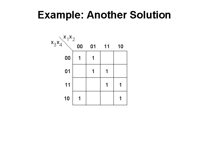
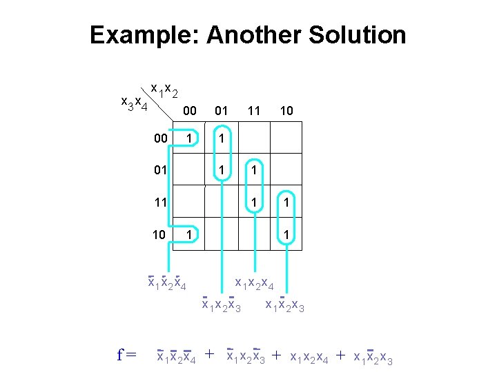
Example: Another Solution x 3 x 4 x 1 x 2 00 00 01 1 11 10 11 1 10 1 1

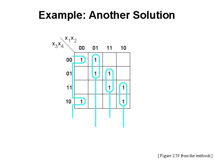
Example: Another Solution x 3 x 4 x 1 x 2 00 00 01 1 11 10 11 1 10 1 1 [ Figure 2. 59 from the textbook ]

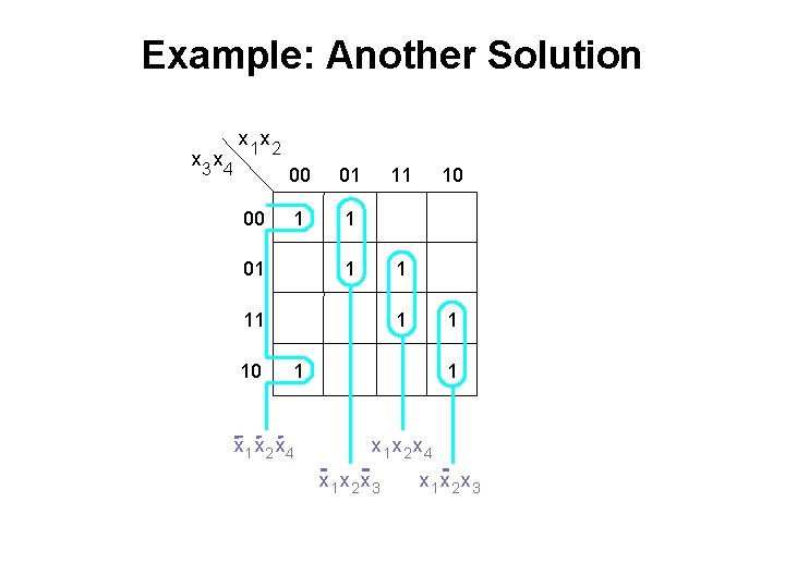
Example: Another Solution x 3 x 4 x 1 x 2 00 00 01 1 1 01 11 10 10 1 1 1 x 1 x 2 x 4 x 1 x 2 x 3

Example: Another Solution x 3 x 4 x 1 x 2 00 00 01 1 1 01 11 10 1 1 x 1 x 2 x 4 x 1 x 2 x 3 f= 10 x 1 x 2 x 4 + x 1 x 2 x 3 + x 1 x 2 x 4 + x 1 x 2 x 3

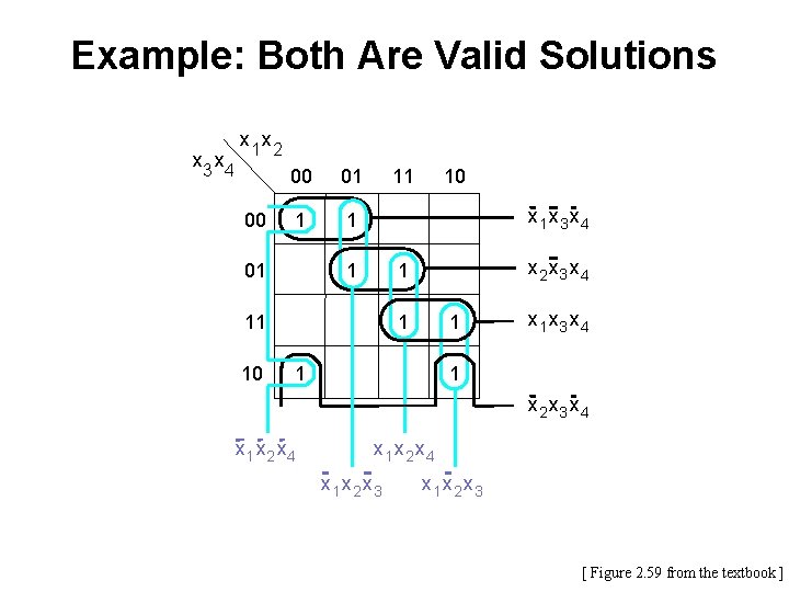
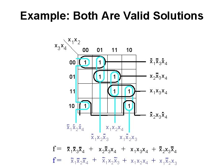
Example: Both Are Valid Solutions x 3 x 4 x 1 x 2 00 00 01 1 1 01 11 x 3 x 4 1 x 2 x 3 x 4 1 11 10 10 1 1 1 x 3 x 4 1 x 2 x 3 x 4 x 1 x 2 x 3 [ Figure 2. 59 from the textbook ]

Example: Both Are Valid Solutions x 3 x 4 x 1 x 2 00 00 01 1 1 01 11 x 3 x 4 1 x 2 x 3 x 4 1 11 10 10 1 x 3 x 4 1 1 1 x 2 x 3 x 4 x 1 x 2 x 3 f= f= + x 1 x 2 x 4 + x 1 x 3 x 4 x 2 x 3 x 4 x 1 x 2 x 3 + x 1 x 3 x 4 + x 2 x 3 x 4 + x 1 x 2 x 3

Minimization of Product-of-Sums Forms

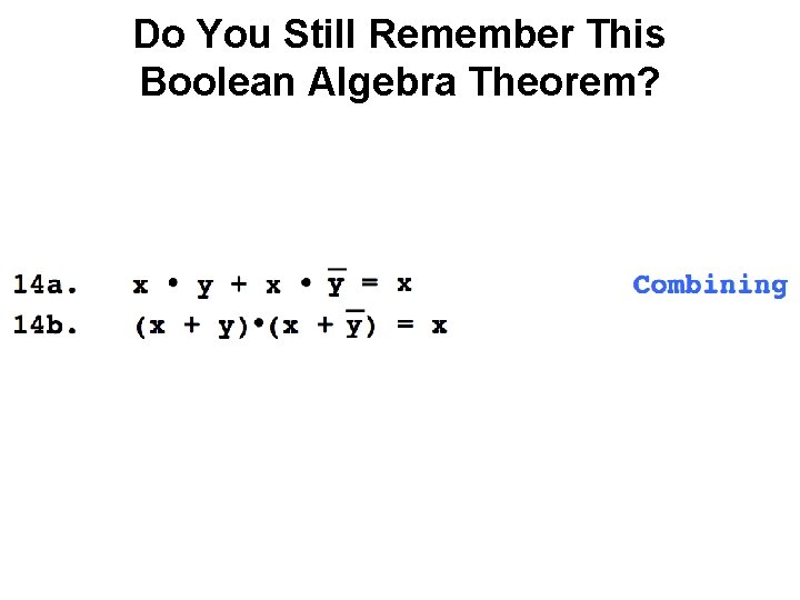
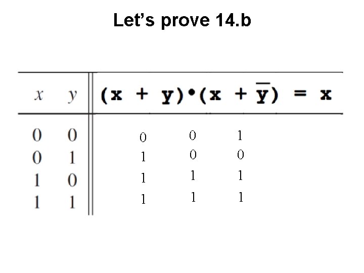
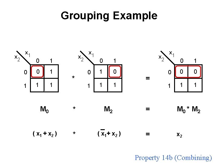
Do You Still Remember This Boolean Algebra Theorem?

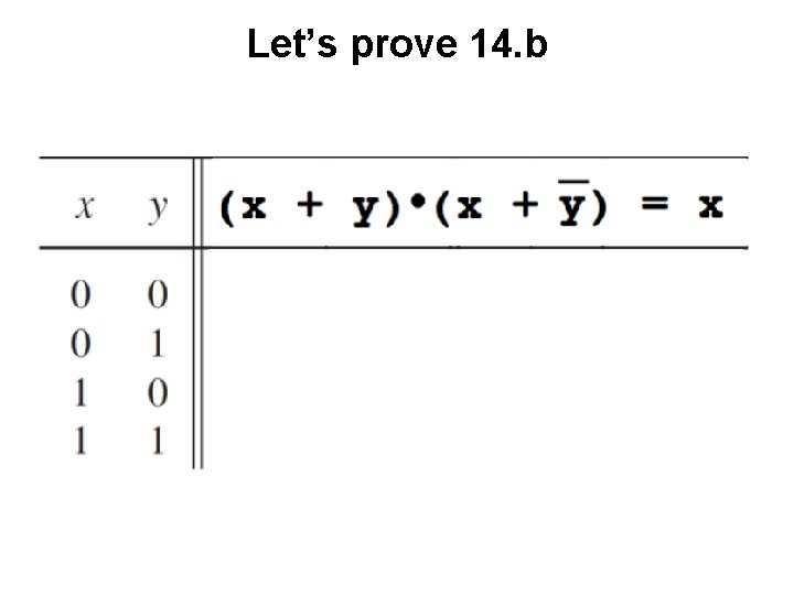
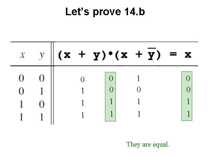
Let’s prove 14. b

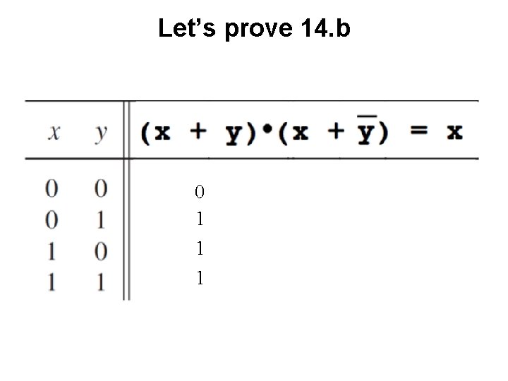
Let’s prove 14. b 0 1 1 1

Let’s prove 14. b 0 1 1 1

Let’s prove 14. b 0 1 1

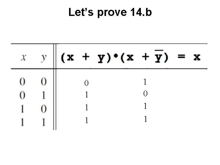
Let’s prove 14. b 0 1 1 0 1 0 0 1 1 1

Let’s prove 14. b 0 1 1 0 1 0 0 1 1 1 They are equal.

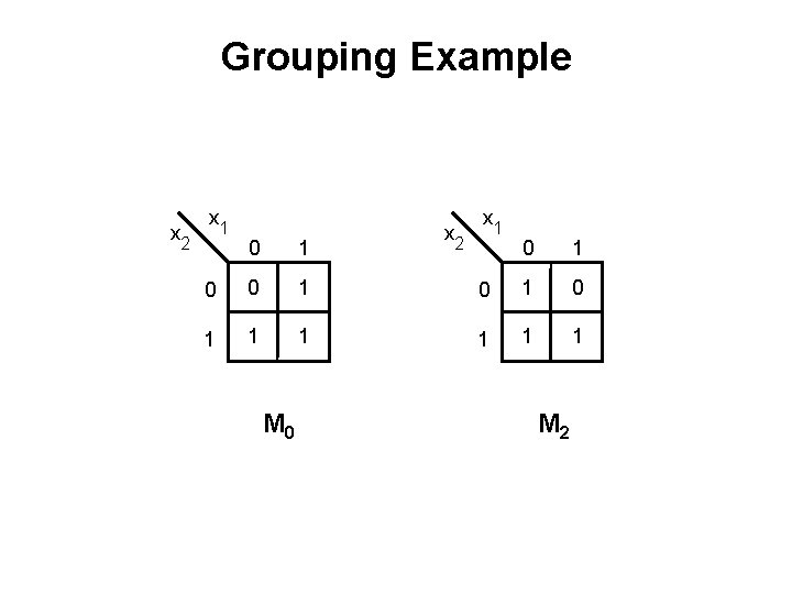
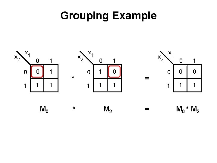
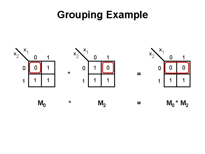
Grouping Example x 2 x 1 0 0 1 1 M 0 x 2 x 1 0 1 0 1 1 1 M 2

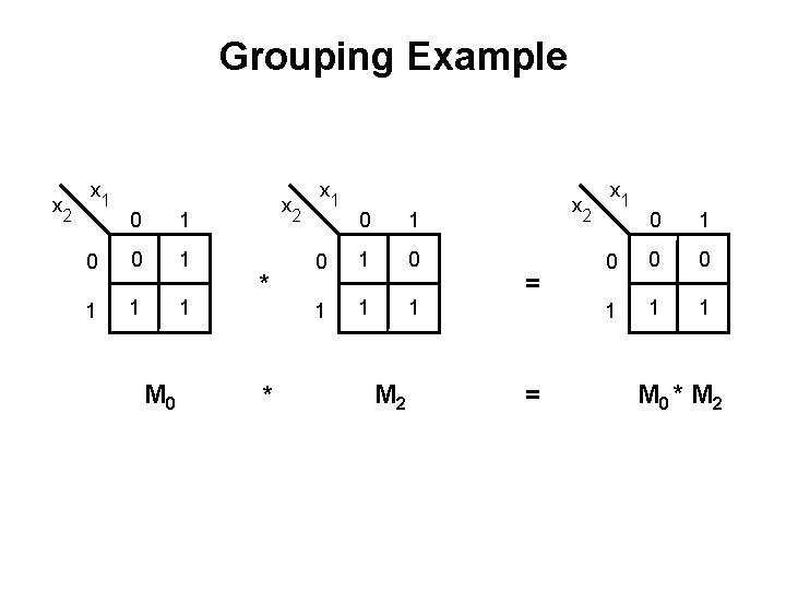
Grouping Example x 2 x 1 0 0 1 1 M 0 x 2 * * x 1 0 1 0 1 1 1 M 2 x 2 = = x 1 0 0 0 1 1 1 M 0 * M 2

Grouping Example x 2 x 1 0 0 1 1 M 0 x 2 * * x 1 0 1 0 1 1 1 M 2 x 2 = = x 1 0 0 0 1 1 1 M 0 * M 2

Grouping Example x 2 x 1 0 0 1 1 M 0 x 2 * * x 1 0 1 0 1 1 1 M 2 x 2 = = x 1 0 0 0 1 1 1 M 0 * M 2

Grouping Example x 2 x 1 0 0 1 1 M 0 ( x 1 + x 2 ) x 2 * * * x 1 0 1 0 1 1 1 M 2 _ ( x 1 + x 2 ) x 2 = x 1 0 0 0 1 1 1 = M 0 * M 2 = x 2 Property 14 b (Combining)

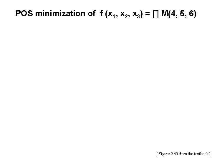
POS minimization of f (x 1, x 2, x 3) = ∏ M(4, 5, 6) [ Figure 2. 60 from the textbook ]

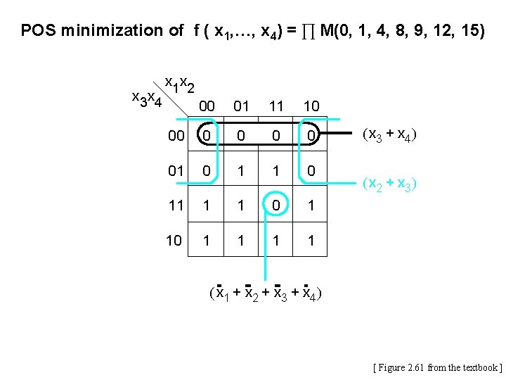
POS minimization of f ( x 1, …, x 4) = ∏ M(0, 1, 4, 8, 9, 12, 15) x 3 x 4 x 1 x 2 00 01 11 10 00 0 0 01 0 11 1 1 0 1 1 1 1 ( x 3 + x 4) ( x 2 + x 3) ( x 1 + x 2 + x 3 + x 4) [ Figure 2. 61 from the textbook ]

Questions?

THE END