CPE 619 Comparing Systems Using Sample Data Aleksandar

CPE 619 Comparing Systems Using Sample Data Aleksandar Milenković The La. CASA Laboratory Electrical and Computer Engineering Department The University of Alabama in Huntsville http: //www. ece. uah. edu/~milenka http: //www. ece. uah. edu/~lacasa

Part III: Probability Theory and Statistics n n n n How to report the performance as a single number? Is specifying the mean the correct way? How to report the variability of measured quantities? What are the alternatives to variance and when are they appropriate? How to interpret the variability? How much confidence can you put on data with a large variability? How many measurements are required to get a desired level of statistical confidence? How to summarize the results of several different workloads on a single computer system? How to compare two or more computer systems using several different workloads? Is comparing the mean sufficient? What model best describes the relationship between two variables? Also, how good is the model? 2

Overview n n n Sample Versus Population Confidence Interval for The Mean Approximate Visual Test One Sided Confidence Intervals for Proportions Sample Size for Determining Mean and proportions 3

Sample n n n Old French word `essample' `sample' and `example' One example theory One sample Definite statement 4

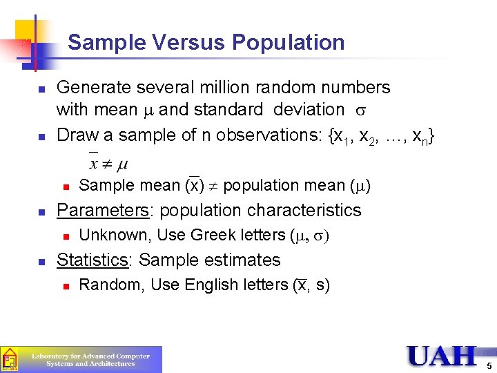
Sample Versus Population n n Generate several million random numbers with mean and standard deviation s Draw a sample of n observations: {x 1, x 2, …, xn} n n Parameters: population characteristics n n Sample mean (x) population mean ( ) Unknown, Use Greek letters ( , s) Statistics: Sample estimates n Random, Use English letters (x, s) 5

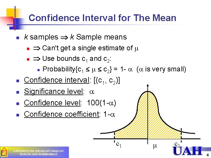
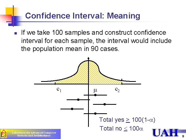
Confidence Interval for The Mean n k samples k Sample means n n n Can't get a single estimate of Use bounds c 1 and c 2: n Probability{c 1 c 2} = 1 - ( is very small) Confidence interval: [(c 1, c 2)] Significance level: Confidence level: 100(1 - ) Confidence coefficient: 1 - c 1 c 2 6

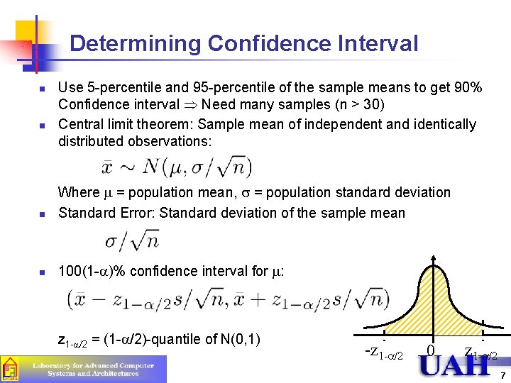
Determining Confidence Interval n n Use 5 -percentile and 95 -percentile of the sample means to get 90% Confidence interval Need many samples (n > 30) Central limit theorem: Sample mean of independent and identically distributed observations: n Where = population mean, s = population standard deviation Standard Error: Standard deviation of the sample mean n 100(1 - )% confidence interval for : z 1 - /2 = (1 - /2)-quantile of N(0, 1) -z 1 - /2 0 z 1 - /2 7

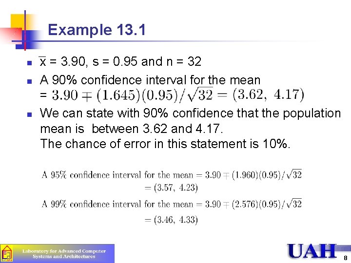
Example 13. 1 n n n x = 3. 90, s = 0. 95 and n = 32 A 90% confidence interval for the mean = We can state with 90% confidence that the population mean is between 3. 62 and 4. 17. The chance of error in this statement is 10%. 8

Confidence Interval: Meaning n If we take 100 samples and construct confidence interval for each sample, the interval would include the population mean in 90 cases. c 1 c 2 Total yes > 100(1 - ) Total no 100 9

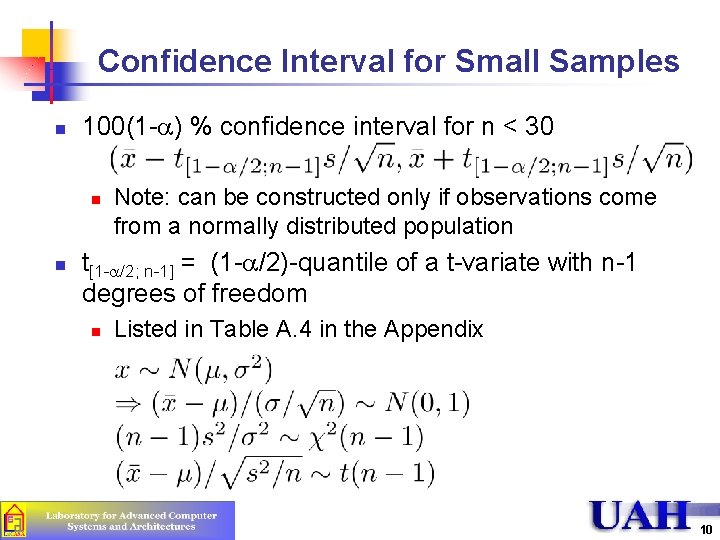
Confidence Interval for Small Samples n 100(1 - ) % confidence interval for n < 30 n n Note: can be constructed only if observations come from a normally distributed population t[1 - /2; n-1] = (1 - /2)-quantile of a t-variate with n-1 degrees of freedom n Listed in Table A. 4 in the Appendix 10

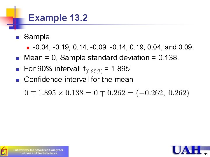
Example 13. 2 n Sample n n -0. 04, -0. 19, 0. 14, -0. 09, -0. 14, 0. 19, 0. 04, and 0. 09. Mean = 0, Sample standard deviation = 0. 138. For 90% interval: t[0. 95; 7] = 1. 895 Confidence interval for the mean 11

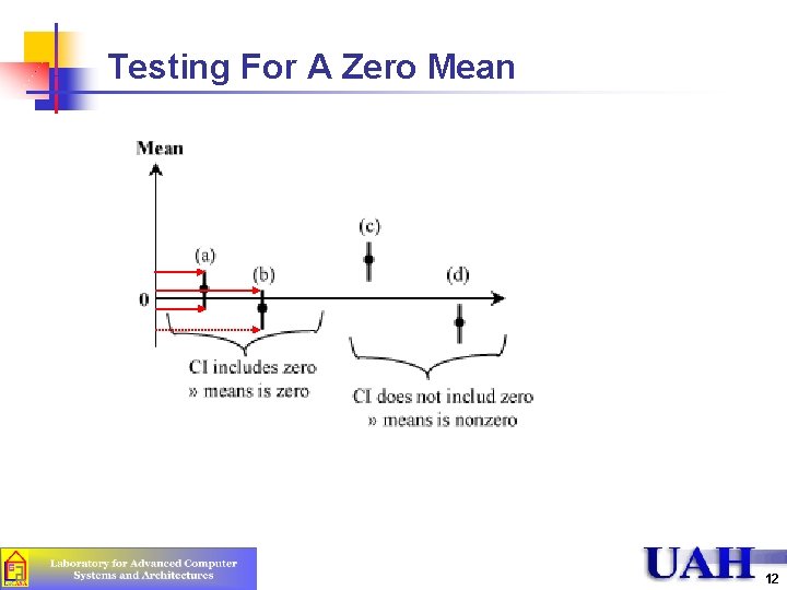
Testing For A Zero Mean 12

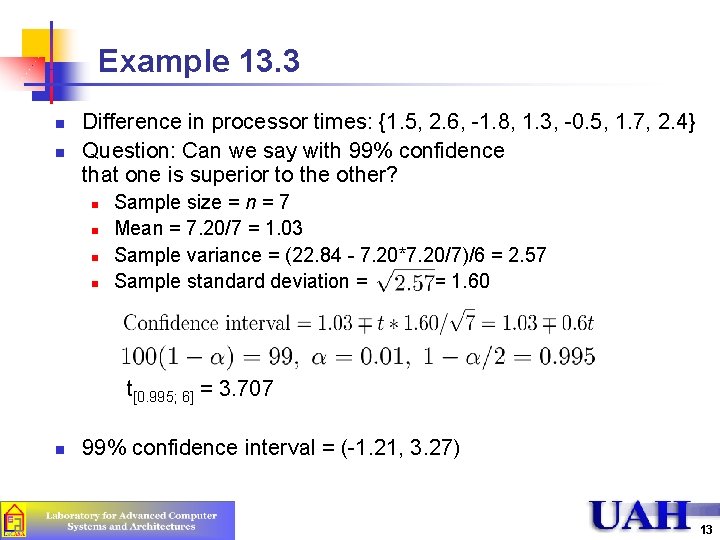
Example 13. 3 n n Difference in processor times: {1. 5, 2. 6, -1. 8, 1. 3, -0. 5, 1. 7, 2. 4} Question: Can we say with 99% confidence that one is superior to the other? n n Sample size = n = 7 Mean = 7. 20/7 = 1. 03 Sample variance = (22. 84 - 7. 20*7. 20/7)/6 = 2. 57 Sample standard deviation = = 1. 60 t[0. 995; 6] = 3. 707 n 99% confidence interval = (-1. 21, 3. 27) 13

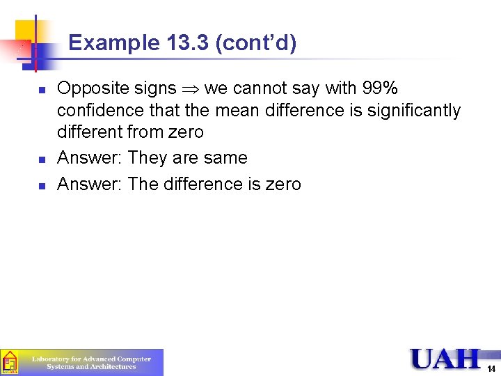
Example 13. 3 (cont’d) n n n Opposite signs we cannot say with 99% confidence that the mean difference is significantly different from zero Answer: They are same Answer: The difference is zero 14

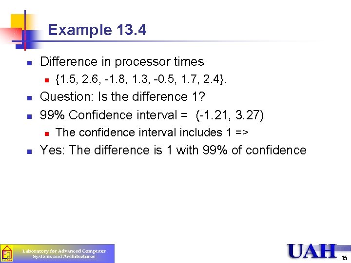
Example 13. 4 n Difference in processor times n n n Question: Is the difference 1? 99% Confidence interval = (-1. 21, 3. 27) n n {1. 5, 2. 6, -1. 8, 1. 3, -0. 5, 1. 7, 2. 4}. The confidence interval includes 1 => Yes: The difference is 1 with 99% of confidence 15

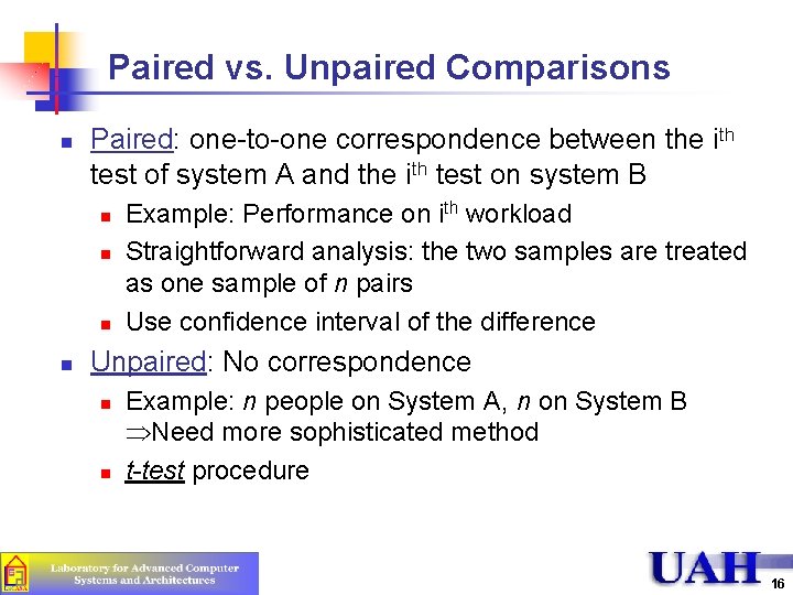
Paired vs. Unpaired Comparisons n Paired: one-to-one correspondence between the ith test of system A and the ith test on system B n n Example: Performance on ith workload Straightforward analysis: the two samples are treated as one sample of n pairs Use confidence interval of the difference Unpaired: No correspondence n n Example: n people on System A, n on System B Need more sophisticated method t-test procedure 16

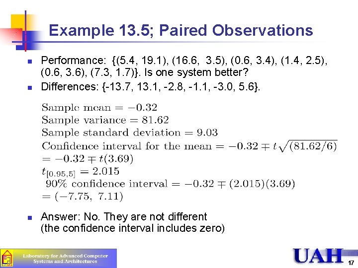
Example 13. 5; Paired Observations n n n Performance: {(5. 4, 19. 1), (16. 6, 3. 5), (0. 6, 3. 4), (1. 4, 2. 5), (0. 6, 3. 6), (7. 3, 1. 7)}. Is one system better? Differences: {-13. 7, 13. 1, -2. 8, -1. 1, -3. 0, 5. 6}. Answer: No. They are not different (the confidence interval includes zero) 17

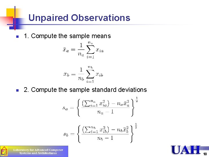
Unpaired Observations n 1. Compute the sample means n 2. Compute the sample standard deviations 18

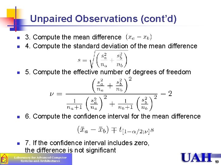
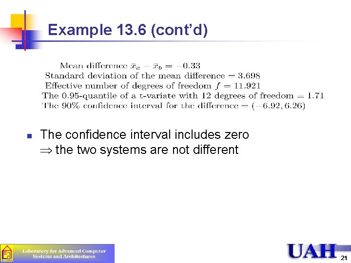
Unpaired Observations (cont’d) n 3. Compute the mean difference 4. Compute the standard deviation of the mean difference n 5. Compute the effective number of degrees of freedom n 6. Compute the confidence interval for the mean difference n n 7. If the confidence interval includes zero, the difference is not significant 19

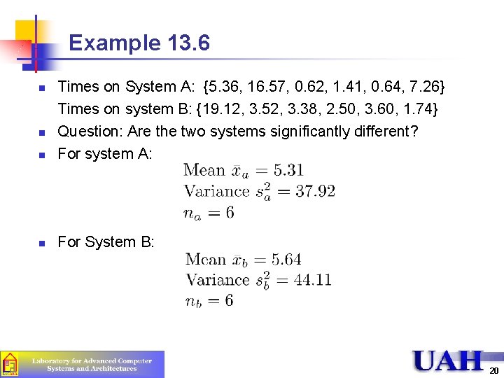
Example 13. 6 n Times on System A: {5. 36, 16. 57, 0. 62, 1. 41, 0. 64, 7. 26} Times on system B: {19. 12, 3. 52, 3. 38, 2. 50, 3. 60, 1. 74} Question: Are the two systems significantly different? For system A: n For System B: n n 20

Example 13. 6 (cont’d) n The confidence interval includes zero the two systems are not different 21

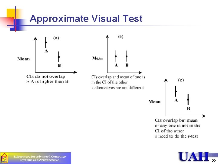
Approximate Visual Test 22

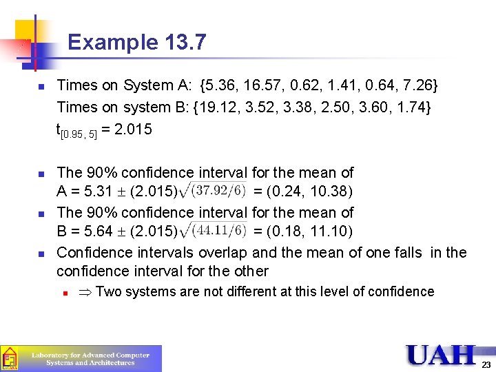
Example 13. 7 n n Times on System A: {5. 36, 16. 57, 0. 62, 1. 41, 0. 64, 7. 26} Times on system B: {19. 12, 3. 52, 3. 38, 2. 50, 3. 60, 1. 74} t[0. 95, 5] = 2. 015 The 90% confidence interval for the mean of A = 5. 31 (2. 015) = (0. 24, 10. 38) The 90% confidence interval for the mean of B = 5. 64 (2. 015) = (0. 18, 11. 10) Confidence intervals overlap and the mean of one falls in the confidence interval for the other n Two systems are not different at this level of confidence 23

What Confidence Level To Use? n n n Need not always be 90% or 95% or 99% Based on the loss that you would sustain if the parameter is outside the range and the gain you would have if the parameter is inside the range Low loss Low confidence level is fine n n n E. g. , lottery of 5 Million, one dollar ticket cost, with probability of winning 10 -7 (one in 10 million) 90% confidence buy 9 million tickets (and pay $9 M) 0. 01% confidence level is fine 50% confidence level may or may not be too low 99% confidence level may or may not be too high 24

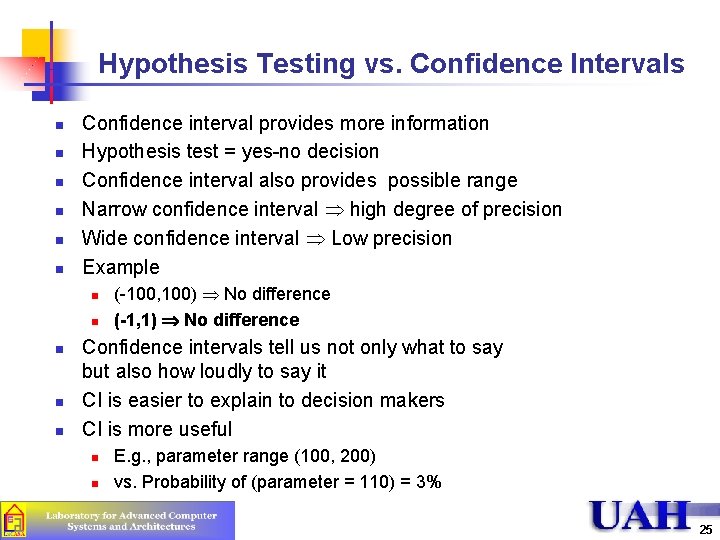
Hypothesis Testing vs. Confidence Intervals n n n Confidence interval provides more information Hypothesis test = yes-no decision Confidence interval also provides possible range Narrow confidence interval high degree of precision Wide confidence interval Low precision Example n n n (-100, 100) No difference (-1, 1) No difference Confidence intervals tell us not only what to say but also how loudly to say it CI is easier to explain to decision makers CI is more useful n n E. g. , parameter range (100, 200) vs. Probability of (parameter = 110) = 3% 25

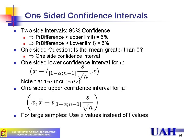
One Sided Confidence Intervals n Two side intervals: 90% Confidence n n n P(Difference > upper limit) = 5% P(Difference < Lower limit) = 5% One sided Question: Is the mean greater than 0? n One side confidence interval n One sided lower confidence interval for : n Note t at 1 - (not 1 - /2) One sided upper confidence interval for : n For large samples: Use z values instead of t values 26

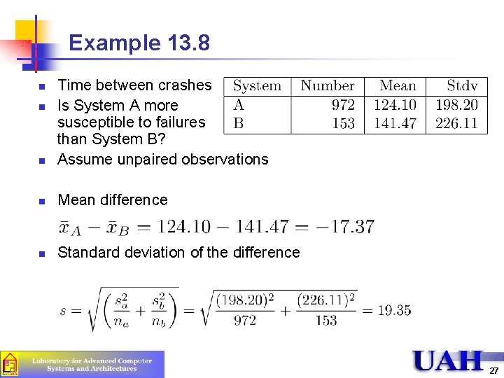
Example 13. 8 n Time between crashes Is System A more susceptible to failures than System B? Assume unpaired observations n Mean difference n Standard deviation of the difference n n 27

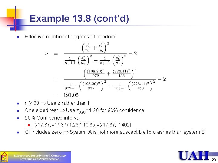
Example 13. 8 (cont’d) n n Effective number of degrees of freedom n > 30 Use z rather than t One sided test Use z 0. 90=1. 28 for 90% confidence 90% Confidence interval n n (-17. 37, -17. 37+1. 28 * 19. 35)=(-17. 37, 7. 402) CI includes zero System A is not more susceptible to crashes than system B 28

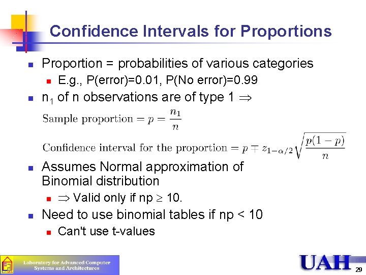
Confidence Intervals for Proportions n Proportion = probabilities of various categories n n 1 of n observations are of type 1 Assumes Normal approximation of Binomial distribution n n E. g. , P(error)=0. 01, P(No error)=0. 99 Valid only if np 10. Need to use binomial tables if np < 10 n Can't use t-values 29

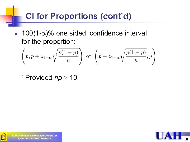
CI for Proportions (cont’d) n 100(1 - )% one sided confidence interval for the proportion: * * Provided np 10. 30

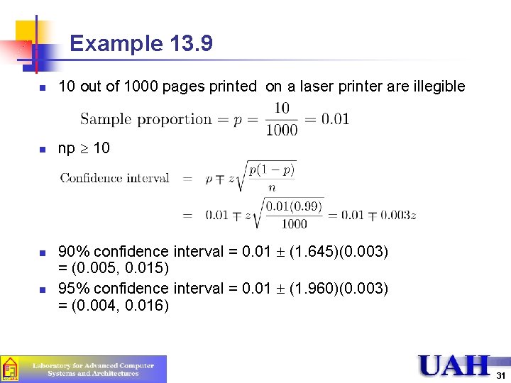
Example 13. 9 n 10 out of 1000 pages printed on a laser printer are illegible n np 10 n n 90% confidence interval = 0. 01 (1. 645)(0. 003) = (0. 005, 0. 015) 95% confidence interval = 0. 01 (1. 960)(0. 003) = (0. 004, 0. 016) 31

Example 13. 9 (cont’d) n At 90% confidence: 0. 5% to 1. 5% of the pages are illegible n n Chances of error = 10% At 95% Confidence: 0. 4% to 1. 6% of the pages are illegible n Chances of error = 5% 32

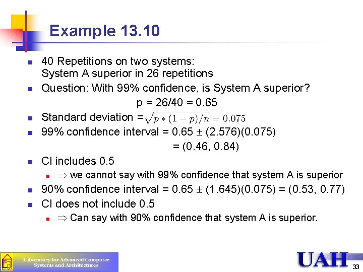
Example 13. 10 n n n 40 Repetitions on two systems: System A superior in 26 repetitions Question: With 99% confidence, is System A superior? p = 26/40 = 0. 65 Standard deviation = 99% confidence interval = 0. 65 (2. 576)(0. 075) = (0. 46, 0. 84) CI includes 0. 5 n n n we cannot say with 99% confidence that system A is superior 90% confidence interval = 0. 65 (1. 645)(0. 075) = (0. 53, 0. 77) CI does not include 0. 5 n Can say with 90% confidence that system A is superior. 33

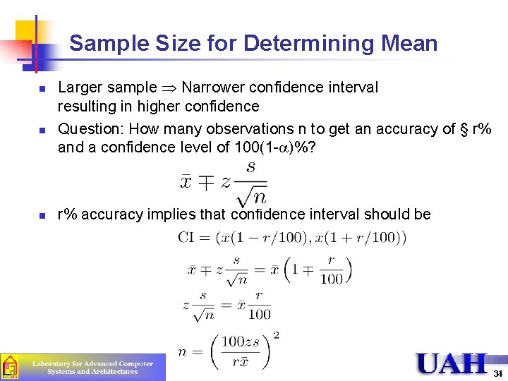
Sample Size for Determining Mean n Larger sample Narrower confidence interval resulting in higher confidence Question: How many observations n to get an accuracy of § r% and a confidence level of 100(1 - )%? r% accuracy implies that confidence interval should be 34

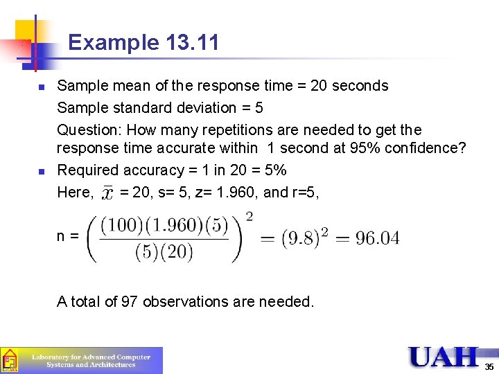
Example 13. 11 n n Sample mean of the response time = 20 seconds Sample standard deviation = 5 Question: How many repetitions are needed to get the response time accurate within 1 second at 95% confidence? Required accuracy = 1 in 20 = 5% Here, = 20, s= 5, z= 1. 960, and r=5, n= A total of 97 observations are needed. 35

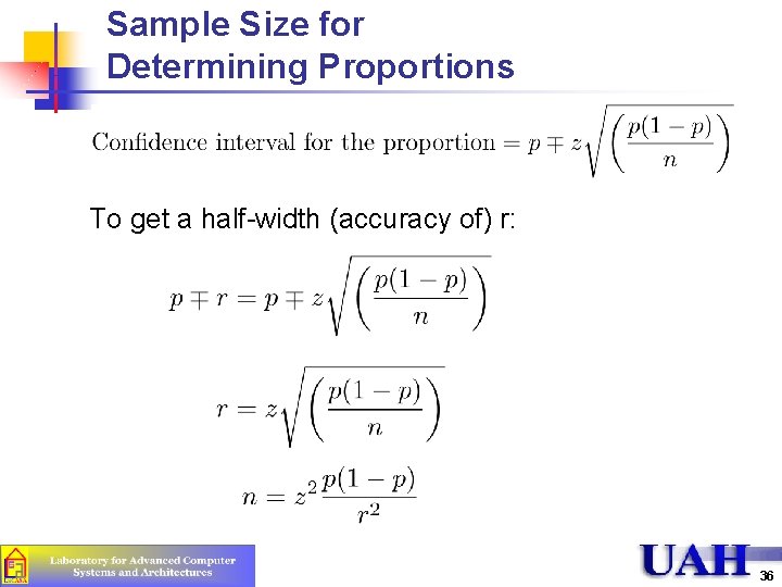
Sample Size for Determining Proportions To get a half-width (accuracy of) r: 36

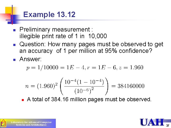
Example 13. 12 n n n Preliminary measurement : illegible print rate of 1 in 10, 000 Question: How many pages must be observed to get an accuracy of 1 per million at 95% confidence? Answer: n A total of 384. 16 million pages must be observed. 37

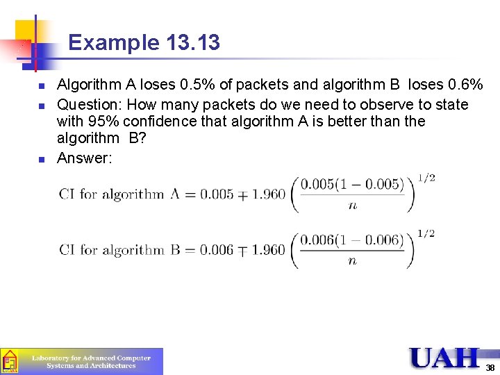
Example 13. 13 n n n Algorithm A loses 0. 5% of packets and algorithm B loses 0. 6% Question: How many packets do we need to observe to state with 95% confidence that algorithm A is better than the algorithm B? Answer: 38

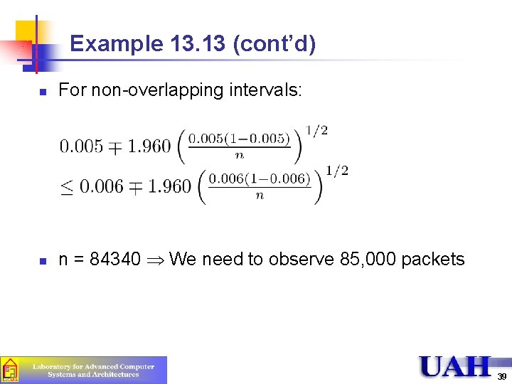
Example 13. 13 (cont’d) n For non-overlapping intervals: n n = 84340 We need to observe 85, 000 packets 39

Summary n n n All statistics based on a sample are random and should be specified with a confidence interval If the confidence interval includes zero, the hypothesis that the population mean is zero cannot be rejected Paired observations Test the difference for zero mean Unpaired observations More sophisticated t-test Confidence intervals apply to proportions too 40

To Do n Read chapter 13 41