CPCS 391 Computer Graphics 1 Instructor Dr Sahar

+ CPCS 391 Computer Graphics 1 Instructor: Dr. Sahar Shabanah Lecture 2

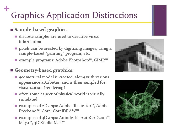
+ Graphics Application Distinctions n n Sample-based graphics: n discrete samples are used to describe visual information n pixels can be created by digitizing images, using a sample-based “painting” program, etc. n example programs: Adobe Photoshop™, GIMP™ Geometry-based graphics: n geometrical model is created, along with various appearance attributes, and is then sampled for visualization (rendering) n often some aspect of physical world is visually simulated n examples of 2 D apps: Adobe Illustrator™, Adobe Freehand™, Corel. DRAW™ n examples of 3 D apps: Autodesk’s Auto. CAD 2010™, Maya™, 3 D Studio Max™ 2

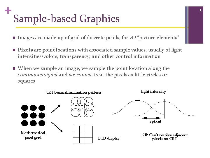
+ 3 Sample-based Graphics n Images are made up of grid of discrete pixels, for 2 D “picture elements” n Pixels are point locations with associated sample values, usually of light intensities/colors, transparency, and other control information n When we sample an image, we sample the point location along the continuous signal and we cannot treat the pixels as little circles or squares CRT beam illumination pattern light intensity 1 pixel Mathematical pixel grid LCD display NB: Can’t resolve adjacent pixels on CRT

+ Sample-based Graphics n Samples created: n n directly in paint-type program, n as a sampling of continuous (analog) visual materials. E. g. , photograph can be sampled (light intensity/color measured at regular intervals) with scanners, cameras n Sample values can also be input numerically (e. g. , with numbers from computed dataset) Once an image is defined as pixel-array, it can be manipulated n Image editing: changes made by user, such as cutting and pasting sections, brush-type tools, and processing selected areas n Image processing: algorithmic operations that are performed on image without user intervention. Includes blurring, sharpening, edge -detection, color balancing, rotating, and warping. Pre-processing step in computer vision 4

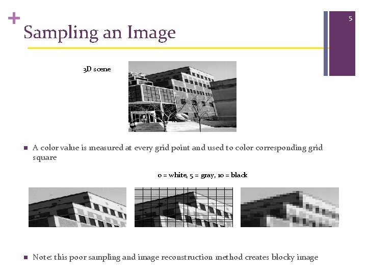
+ Sampling an Image 3 D scene n A color value is measured at every grid point and used to color corresponding grid square 0 = white, 5 = gray, 10 = black n Note: this poor sampling and image reconstruction method creates blocky image 5

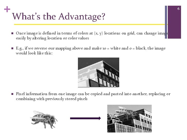
+ What’s the Advantage? n Once image is defined in terms of colors at (x, y) locations on grid, can change image easily by altering location or color values n E. g. , if we reverse our mapping above and make 10 = white and 0 = black, the image would look like this: n Pixel information from one image can be copied and pasted into another, replacing or combining with previously stored pixels 6

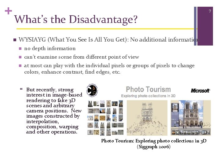
+ What’s the Disadvantage? n WYSIAYG (What You See Is All You Get): No additional information n no depth information n can’t examine scene from different point of view n at most can play with the individual pixels or groups of pixels to change colors, enhance contrast, find edges, etc. But recently, strong interest in image-based rendering to fake 3 D scenes and arbitrary camera positions. New images constructed by interpolation, composition, warping and other operations. Photo Tourism: Exploring photo collections in 3 D (Siggraph 2006) 7

+ Geometry-Based Graphics n Geometry-based graphics applications store mathematical descriptions, or “models, ” of geometric elements (lines, polygons, polyhedrons…) and associated attributes (e. g. , color, material properties). Elements are primitive geometric shapes, primitives for short n Images created as pixel arrays (via sampling of geometry) for viewing, but not stored as part of model. Images of many different views are generated from same model n Users cannot usually work directly with individual pixels in geometry-based programs; as user manipulates geometric elements, program resamples and redisplays elements n Increasingly rendering combines geometric and sample-based graphics, both as performance hack and to increase quality of final product 8

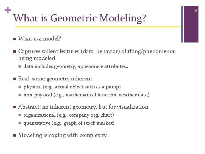
+ What is Geometric Modeling? n What is a model? n Captures salient features (data, behavior) of thing/phenomenon being modeled n n data includes geometry, appearance attributes… Real: some geometry inherent n physical (e. g. , actual object such as a pump) n non-physical (e. g. , mathematical function, weather data) Abstract: no inherent geometry, but for visualization n organizational (e. g. , company org. chart) n quantitative (e. g. , graph of stock market) Modeling is coping with complexity 9

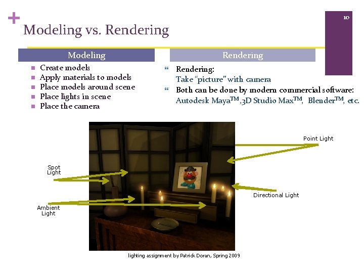
+ 10 Modeling vs. Rendering Modeling n n n Rendering Create models Apply materials to models Place models around scene Place lights in scene Place the camera Rendering: Take “picture” with camera Both can be done by modern commercial software: Autodesk Maya. TM , 3 D Studio Max. TM, Blender. TM, etc. Point Light Spot Light Directional Light Ambient Light lighting assignment by Patrick Doran, Spring 2009

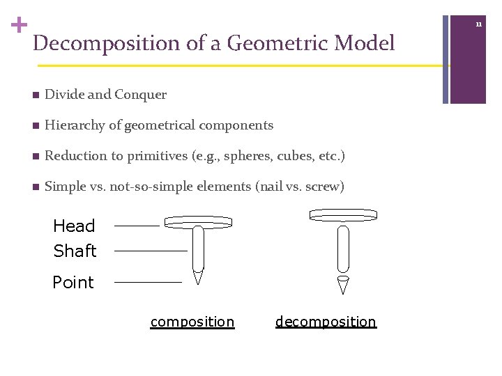
+ Decomposition of a Geometric Model n Divide and Conquer n Hierarchy of geometrical components n Reduction to primitives (e. g. , spheres, cubes, etc. ) n Simple vs. not-so-simple elements (nail vs. screw) Head Shaft Point composition decomposition 11

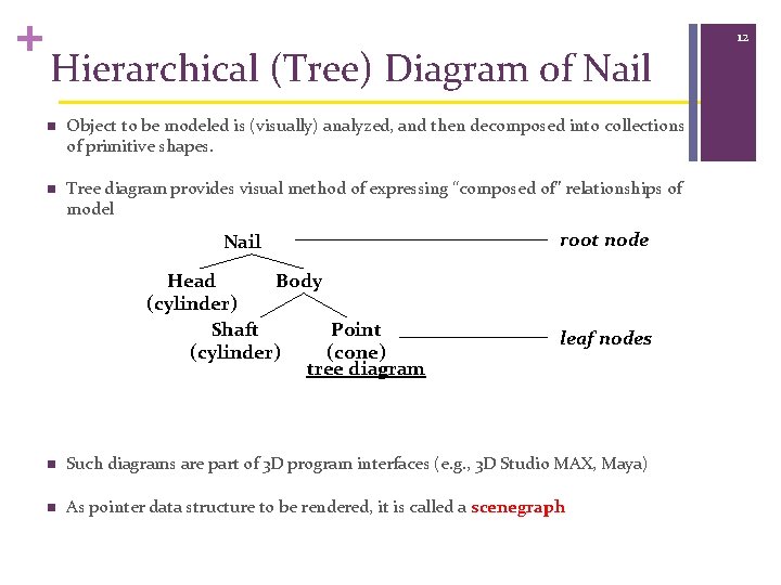
+ Hierarchical (Tree) Diagram of Nail n Object to be modeled is (visually) analyzed, and then decomposed into collections of primitive shapes. n Tree diagram provides visual method of expressing “composed of” relationships of model Nail Head Body (cylinder) Shaft Point (cylinder) (cone) tree diagram root node leaf nodes n Such diagrams are part of 3 D program interfaces (e. g. , 3 D Studio MAX, Maya) n As pointer data structure to be rendered, it is called a scenegraph 12

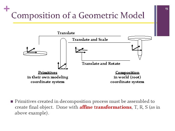
+ Composition of a Geometric Model Translate and Scale Translate and Rotate Primitives in their own modeling coordinate system n Composition in world (root) coordinate system Primitives created in decomposition process must be assembled to create final object. Done with affine transformations, T, R, S (as in above example). 13

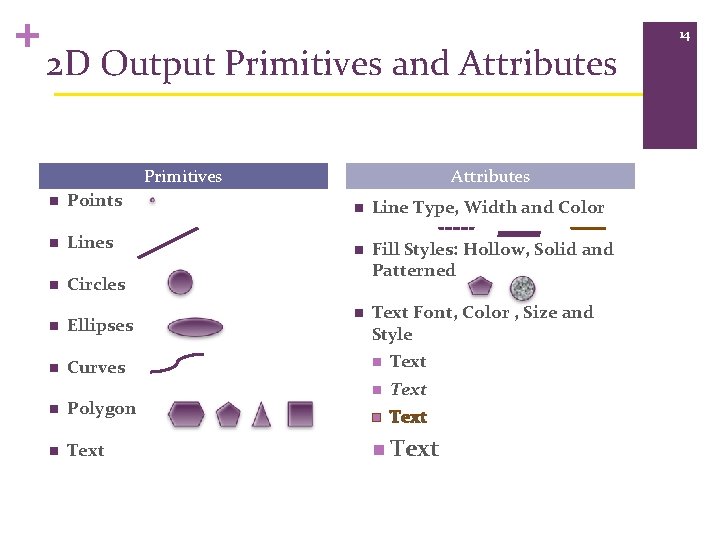
+ 2 D Output Primitives and Attributes Primitives Attributes n Points n Line Type, Width and Color n Lines n n Circles Fill Styles: Hollow, Solid and Patterned n Ellipses n Text Font, Color , Size and Style n Curves n Polygon n Text n Text 14

+ Scan conversion Algorithms n Primitives and Attributes n Why Scan Conversion? n Algorithms for Scan Conversion: n Lines n Circles n Ellipses n Filling n Polygons 15

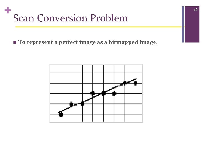
+ Scan Conversion Problem n To represent a perfect image as a bitmapped image. 16

+ Line Drawing Algorithms n Lines are used a lot - want to get them right. n Lines should appear straight, not jagged. n Horizontal, vertical and diagonal easy, others difficult n Lines should terminate accurately. n Lines should have constant density. n Line density should be independent of line length or angle. n Lines should be drawn rapidly. n Efficient algorithms. 17

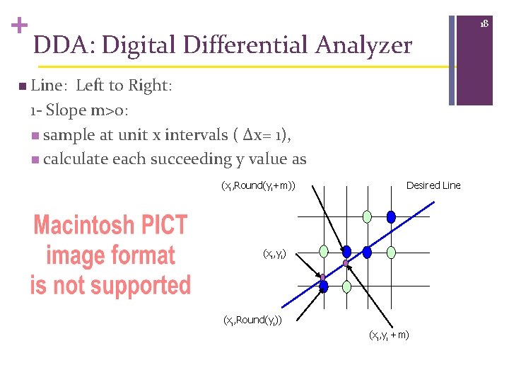
+ DDA: Digital Differential Analyzer n Line: Left to Right: 1 - Slope m>0: n sample at unit x intervals ( Δx= 1), n calculate each succeeding y value as (xi, Round(yi+m)) Desired Line (xi, yi) (xi, Round(yi)) (xi, yi +m) 18

+ 19 DDA 2 - Slope m<0: n sample at unit y intervals ( Δy= 1), n calculate each succeeding x value as n Line: from Right to Left 3 - Slope m> 0: 4 - Slope m< 0:

+ 20 DDA Advantages n Faster than brute force. n Based on Calculating either ∆x or ∆y. n Mathematically defined well Disadvantages n Floating n Round n Time point off error. consuming arithmetic

+ Bresenhams Line Algorithm n Accurate n Efficient n Integer n Uses Calculations Symmetry for other lines n Adapted n It to display circles, ellipses and curves has been proven that the algorithm gives an optimal fit for lines 21

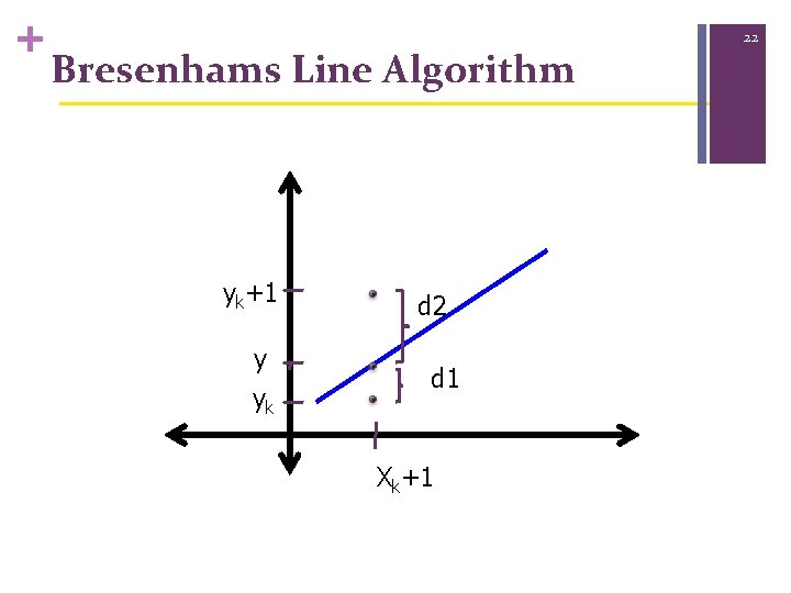
+ Bresenhams Line Algorithm yk+1 y yk d 2 d 1 Xk+1 22

+ Bresenhams Line Algorithm 23

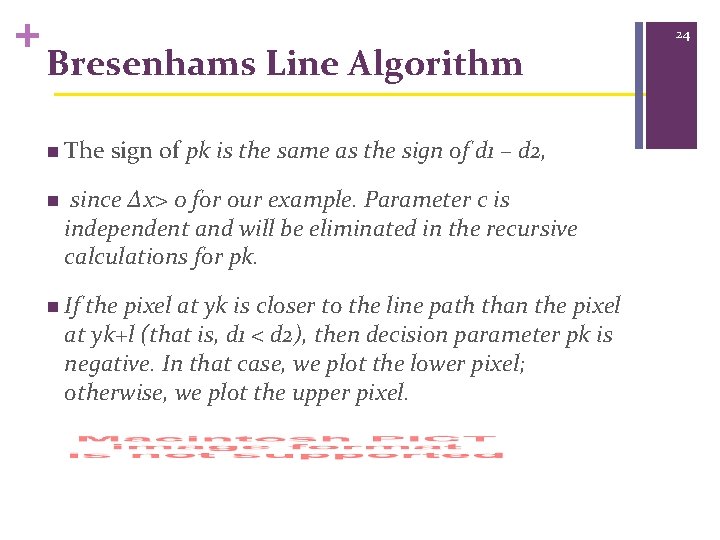
+ Bresenhams Line Algorithm n The n sign of pk is the same as the sign of d 1 – d 2, since Δx> 0 for our example. Parameter c is independent and will be eliminated in the recursive calculations for pk. n If the pixel at yk is closer to the line path than the pixel at yk+l (that is, d 1 < d 2), then decision parameter pk is negative. In that case, we plot the lower pixel; otherwise, we plot the upper pixel. 24

+ Bresenhams Line Algorithm n This recursive calculation of decision parameters is performed at each integer x position, starting at the left coordinate endpoint of the line. The first parameter, po is evaluated from Eq. 3 -12 at the starting pixel position (xo, yo) and with m evaluated as Δy/Δx: 25

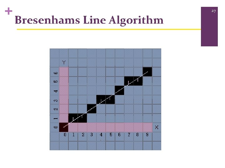
+ Bresenhams Line Drawing Algorithm 1. Input the two line endpoints, store the left endpoint (x 0, y 0). 2. Plot the first point (x 0, y 0). 3. Calculate constants ∆x, ∆y, and 2∆y - 2∆x and 2∆y, get starting values for decision parameter pk, p 0=2∆y-∆x 4. At each xk along the line, starting at k = 0, do the following test: if pk < 0, the next point to plot is(xk+1, yk) pk+1 = pk + 2∆y else, the next point to plot is(xk+1, yk+1) pk+1=pk +2∆y-2∆x 5. Repeat step 4. ∆x times. 26

+ Bresenhams Line Algorithm 27

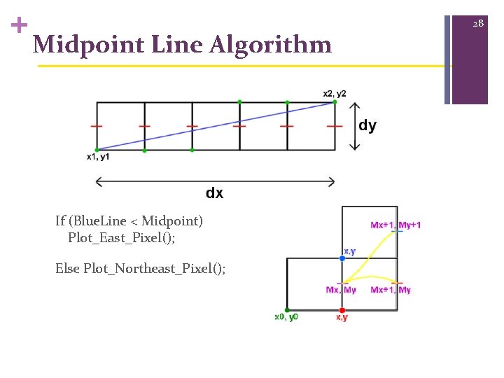
+ Midpoint Line Algorithm If (Blue. Line < Midpoint) Plot_East_Pixel(); Else Plot_Northeast_Pixel(); 28

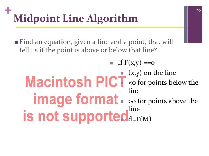
+ Midpoint Line Algorithm 29 n Find an equation, given a line and a point, that will tell us if the point is above or below that line? n If F(x, y) ==0 n (x, y) on the line n <0 for points below the line n >0 for points above the line n d=F(M)

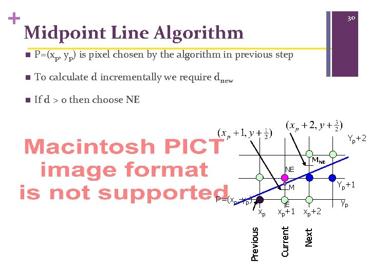
30 Midpoint Line Algorithm n P=(xp, yp) is pixel chosen by the algorithm in previous step n To calculate d incrementally we require dnew n If d > 0 then choose NE Yp+2 NE MNE Yp+1 M xp+1 xp+2 Next xp E Current P=(xp, yp) Previous + yp

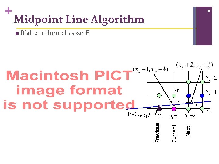
31 Midpoint Line Algorithm d < 0 then choose E Yp+2 NE Yp+1 M xp xp+1 xp+2 Next P=(xp, yp) E ME Current n If Previous + yp

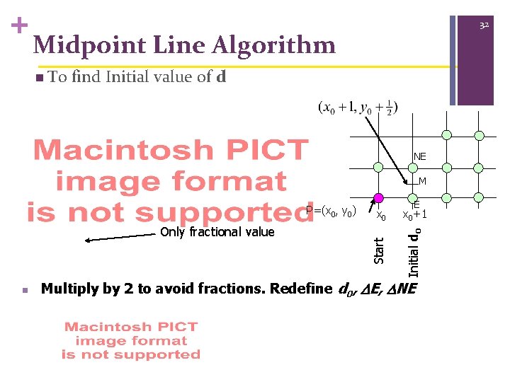
+ 32 Midpoint Line Algorithm n To find Initial value of d NE M n x 0+1 Initial do Only fractional value E Start P=(x 0, y 0) Multiply by 2 to avoid fractions. Redefine d 0, E, NE

+ Midpoint Line Algorithm n Midpoint: Looks at which side of the line the mid point falls on. n Bresenham: in errors. n It Looks at sign of scaled difference has been proven that Midpoint is equivalent to Bresenhams for lines. 33