CPC Morphing Technique Rain Gauge Data Merged with

*CPC Morphing Technique Rain Gauge Data Merged with CMORPH* Yields: RMORPH John Janowiak Climate Prediction Center/NCEP/NWS Jianyin Liang China Meteorological Agency Pingping Xie Climate Prediction Center/NCEP/NWS Robert Joyce CPC / RS Information Systems IPWG-3 -- Melbourne, Australia October 24, 2006

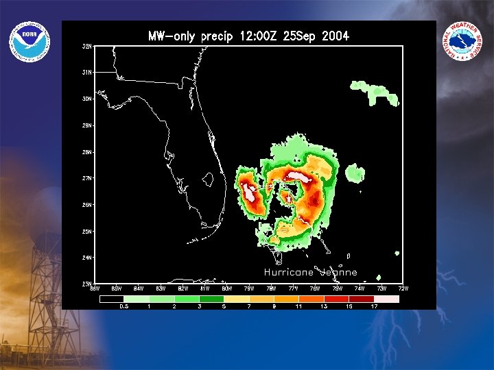
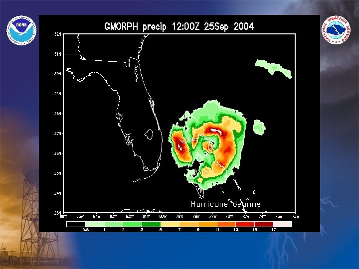
(microwave) ? ? 1. 5 hours apart GPM offers 3 -hr sampling … to get finer temporal sampling … take advantage of 30 -minute sampling afforded by Geo-IR data Premise: Error in using IR to interpolate precip. features identified by PMW < Error in deriving precip. directly from IR So avoid deriving precipitation estimates directly from IR …

(microwave) ? ? 1. 5 hours apart Derive motion vectors from ½ hourly IR Apply motion to PMW-derived precipitation “Morph” (Joyce et al. , J. Hydromet, 2004)

Biases in Satellite Estimates

Gauge-CMORPH Merging Algorithm Step 1: Bias Correction • Assumptions - Biases relatively stable over a region and time - Biases can be approximated as ratios between the estimates & gauges • Procedures - Performed once a day using data for all 24 hourly slots - Each day: RATIO = GAUGE / CMORPH (last 30 days; each gauge) - Optimal Interpolation (OI) technique (Gandin 1965) applied to ratios - “Un”biased CMORPH: CMORPH x RATIOanalyzed

Gauge-CMORPH Merging Algorithm Step 2: Combining Gauge & Satellite Data Bias-corrected satellite estimates and gauge data combined via Optimum Interpolation Technique (“OI”) - Bias-corrected satellite estimates used as first-guess - Gauge data are incorporated - Relative weighting at a grid box is a function of: - quality of satellite estimates at the grid box; - density of local gauge network density

Proof-of-Concept: Guang-Dong Province over Southern China Topography Tibet plateau Guang-Dong South China Sea

Hourly precipitation reports from 394 stations over ~150, 000 km 2 (~380 km 2/gauge)

An Example for 03 Z, May 5, 2005 GAUGE ONLY BIAS CORRECTED ORIGINAL CMORPH MERGED

An Example for 03 Z, May 5, 2005 GAUGE ONLY BIAS CORRECTED ORIGINAL CMORPH MERGED

Mean Precipitation from April 1 – June 30, 2005 GAUGE ONLY BIAS CORRECTED ORIGINAL CMORPH MERGED

Hourly Gauge-Satellite Merged

PDF of Hourly Precipitation • Frequency of No-Rain Events • Gauge Station: 83. 9% • Gauge Analysis: 81. 5% • Original CMORPH: 77. 3% • Gauge-CMORPH Merged: 83. 3% • Frequency of Events with Rain for April - June, 2005

Dense Gauge Locations: Disaggregate Gauge Data Use hourly CMORPH to partition daily gauge amounts into hourly amounts (i. e. “disaggregate”) - United States - Australia - China?

Valid for 24 hrs ending 12 z August 8, 2006

Valid for 24 hrs ending 12 z August 8, 2006 Daily sum of hourly amounts -Daily RMORPH constrained to daily gauge amount - Gauge data partitioned into hourly amounts -Spurious coverage of light gauge amounts reduced

Where to from Here? 1. Transition regional prototype to global 2. Experiment with OI tuning parameters 3. Cross-validation testing 4. Explore bias-adjustment for oceanic precip - Normalize estimates to TRMM “ 2 B 31” (TMI/PR) - ATLAS buoys? - Radar?

Thanks for listening

An Example for 03 Z, May 5, 2005 GAUGE ONLY BIAS CORRECTED ORIGINAL CMORPH MERGED

An Example for 03 Z, May 5, 2005 GAUGE ONLY BIAS CORRECTED ORIGINAL CMORPH MERGED

(microwave) (in time)

Observed (in time)

2/3 1/3 + + 1/3 2/3