Cox Regression II Monday Gut Check Problem n

Cox Regression II

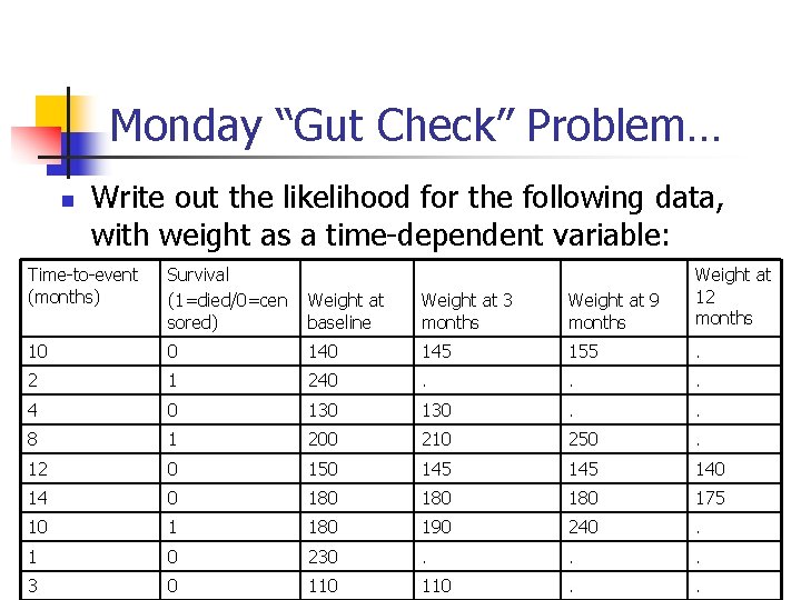
Monday “Gut Check” Problem… n Write out the likelihood for the following data, with weight as a time-dependent variable: Time-to-event (months) Survival (1=died/0=cen sored) Weight at baseline Weight at 3 months Weight at 9 months Weight at 12 months 10 0 145 155 . 2 1 240 . . . 4 0 130 . . 8 1 200 210 250 . 12 0 150 145 140 14 0 180 180 175 10 1 180 190 240 . 1 0 230 . . . 3 0 110 . .

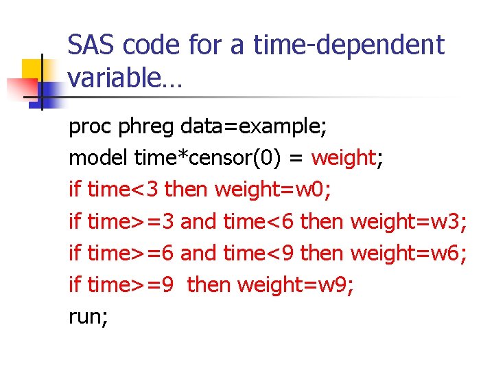
SAS code for a time-dependent variable… proc phreg data=example; model time*censor(0) = weight; if time<3 then weight=w 0; if time>=3 and time<6 then weight=w 3; if time>=6 and time<9 then weight=w 6; if time>=9 then weight=w 9; run;

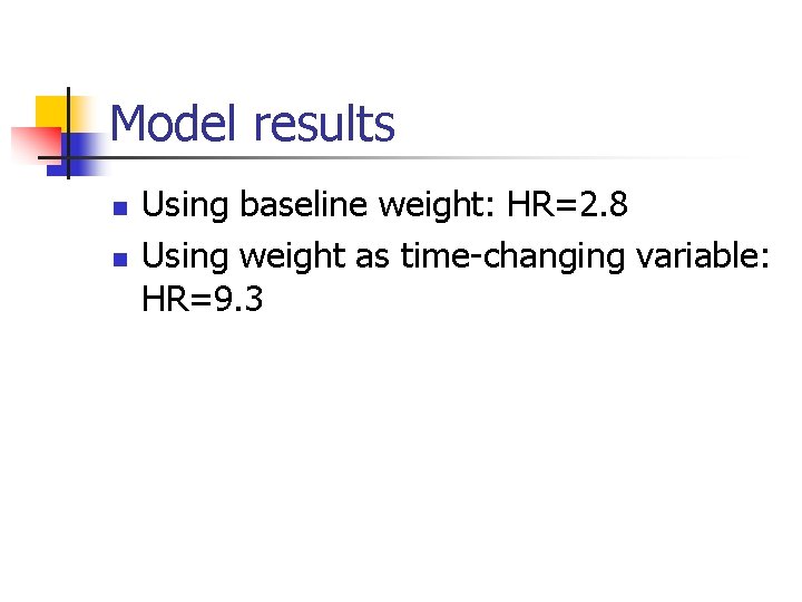
Model results n n Using baseline weight: HR=2. 8 Using weight as time-changing variable: HR=9. 3

1. Stratification Violations of PH assumption can be resolved by: • Adding time*covariate interaction • Adding other time-dependent version of the covariate • Stratification

Stratification • Different stratum are allowed to have different baseline hazard functions. • Hazard functions do not need to be parallel between different stratum. • Essentially results in a “weighted” hazard ratio being estimated: weighted over the different strata. • Useful for “nuisance” confounders (where you do not care to estimate the effect). • Assumes no interaction between the stratification variable and the main predictors.

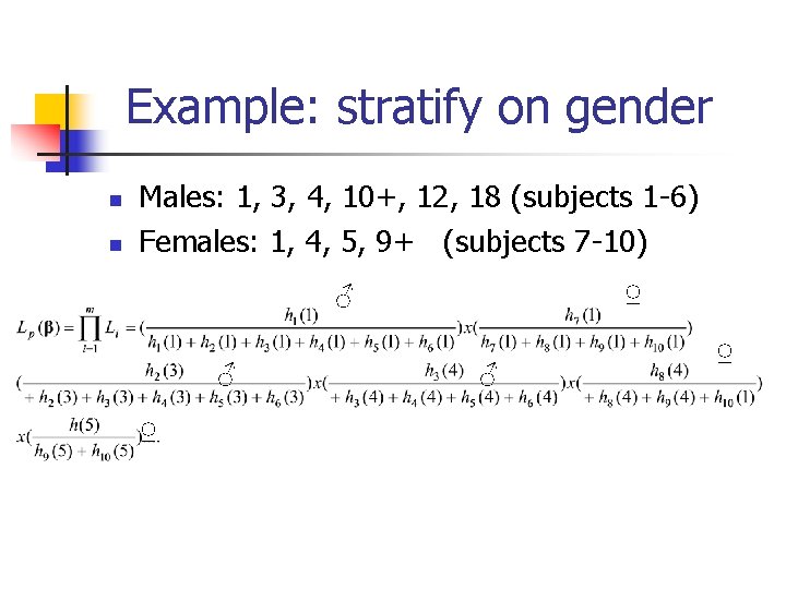
Example: stratify on gender n n Males: 1, 3, 4, 10+, 12, 18 (subjects 1 -6) Females: 1, 4, 5, 9+ (subjects 7 -10) ♂ ♂ ♀ ♀ ♂ ♀

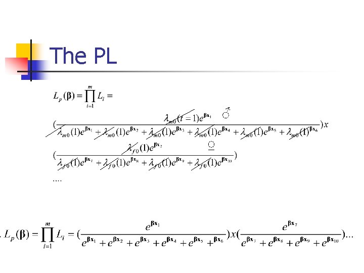
The PL ♂ ♀

2. Using age as the time-scale in Cox Regression n n Age is a common confounder in Cox Regression, since age is strongly related to death and disease. You may control for age by adding baseline age as a covariate to the Cox model. A better strategy for large-scale longitudinal surveys, such as NHANES, is to use age as your time-scale (rather than time-in-study). You may additionally stratify on birth cohort to control for cohort effects.

Age as time-scale n n n The risk set becomes everyone who was at risk at a certain age rather than at a certain event time. The risk set contains everyone who was still event-free at the age of the person who had the event. Requires enough people at risk at all ages (such as in a large-scale, longitudinal survey).

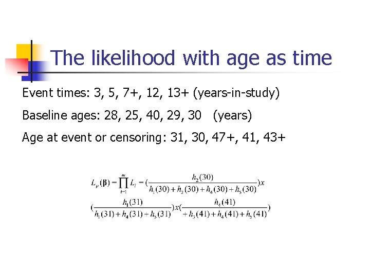
The likelihood with age as time Event times: 3, 5, 7+, 12, 13+ (years-in-study) Baseline ages: 28, 25, 40, 29, 30 (years) Age at event or censoring: 31, 30, 47+, 41, 43+

3. Residuals n n Residuals are used to investigate the lack of fit of a model to a given subject. For Cox regression, there’s no easy analog to the usual “observed minus predicted” residual of linear regression

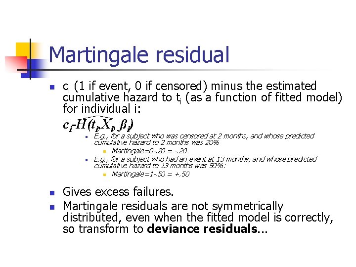
Martingale residual n ci (1 if event, 0 if censored) minus the estimated cumulative hazard to ti (as a function of fitted model) for individual i: ci-H(ti, Xi, ßi) n n E. g. , for a subject who was censored at 2 months, and whose predicted cumulative hazard to 2 months was 20% n Martingale=0 -. 20 = -. 20 E. g. , for a subject who had an event at 13 months, and whose predicted cumulative hazard to 13 months was 50%: n Martingale=1 -. 50 = +. 50 Gives excess failures. Martingale residuals are not symmetrically distributed, even when the fitted model is correctly, so transform to deviance residuals. . .

Deviance Residuals n n The deviance residual is a normalized transform of the martingale residual. These residuals are much more symmetrically distributed about zero. Observations with large deviance residuals are poorly predicted by the model.

Deviance Residuals n n Behave like residuals from ordinary linear regression Should be symmetrically distributed around 0 and have standard deviation of 1. 0. Negative for observations with longer than expected observed survival times. Plot deviance residuals against covariates to look for unusual patterns.

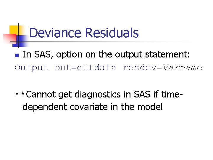
Deviance Residuals In SAS, option on the output statement: Output out=outdata resdev=Varname n **Cannot get diagnostics in SAS if timedependent covariate in the model

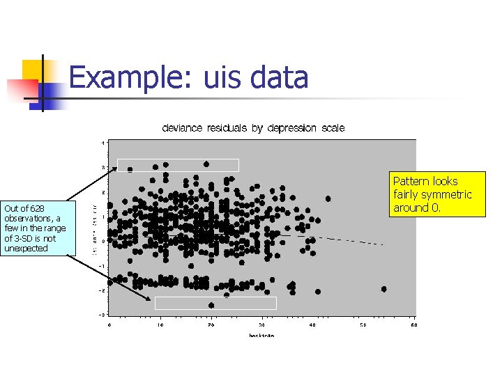
Example: uis data Out of 628 observations, a few in the range of 3 -SD is not unexpected Pattern looks fairly symmetric around 0.

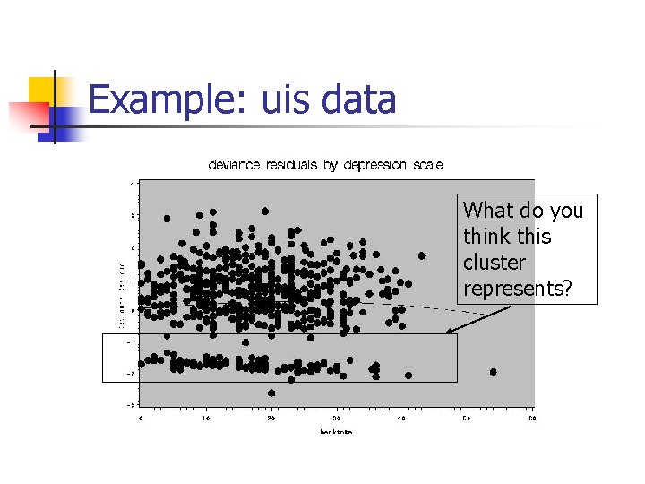
Example: uis data What do you think this cluster represents?

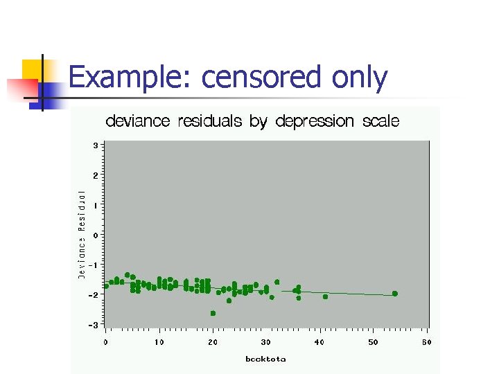
Example: censored only

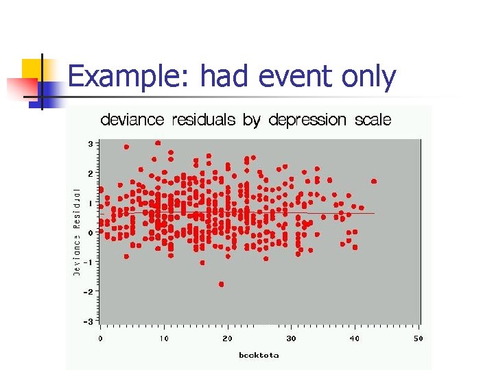
Example: had event only

Schoenfeld residuals n Schoenfeld (1982) proposed the first set of residuals for use with Cox regression packages n n n Schoenfeld D. Residuals for the proportional hazards regresssion model. Biometrika, 1982, 69(1): 239 -241. Instead of a single residual for each individual, there is a separate residual for each individual for each covariate Note: Schoenfeld residuals are not defined for censored individuals.

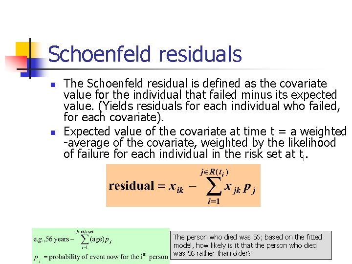
Schoenfeld residuals n n The Schoenfeld residual is defined as the covariate value for the individual that failed minus its expected value. (Yields residuals for each individual who failed, for each covariate). Expected value of the covariate at time ti = a weighted -average of the covariate, weighted by the likelihood of failure for each individual in the risk set at ti. The person who died was 56; based on the fitted model, how likely is it that the person who died was 56 rather than older?

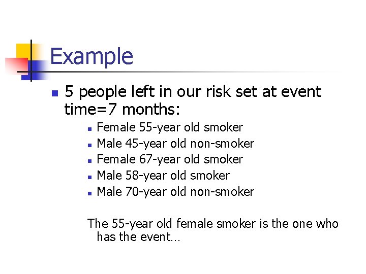
Example n 5 people left in our risk set at event time=7 months: n n n Female 55 -year old smoker Male 45 -year old non-smoker Female 67 -year old smoker Male 58 -year old smoker Male 70 -year old non-smoker The 55 -year old female smoker is the one who has the event…

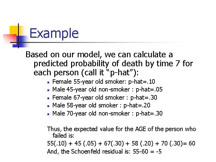
Example Based on our model, we can calculate a predicted probability of death by time 7 for each person (call it “p-hat”): n n n Female 55 -year old smoker: p-hat=. 10 Male 45 -year old non-smoker : p-hat=. 05 Female 67 -year old smoker : p-hat=. 30 Male 58 -year old smoker : p-hat=. 20 Male 70 -year old non-smoker : p-hat=. 30 Thus, the expected value for the AGE of the person who failed is: 55(. 10) + 45 (. 05) + 67(. 30) + 58 (. 20) + 70 (. 30)= 60 And, the Schoenfeld residual is: 55 -60 = -5

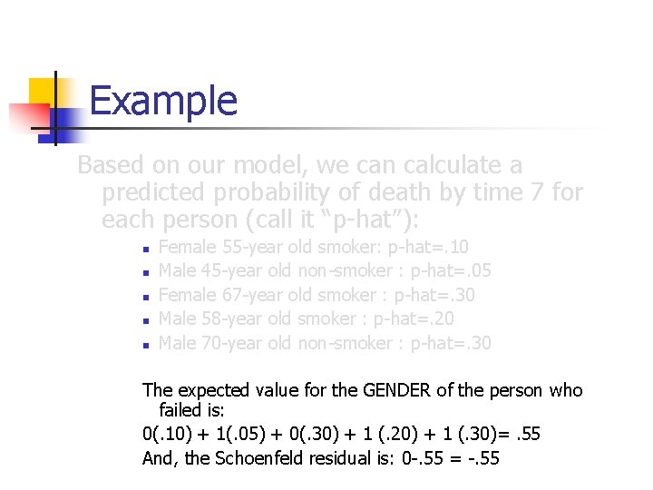
Example Based on our model, we can calculate a predicted probability of death by time 7 for each person (call it “p-hat”): n n n Female 55 -year old smoker: p-hat=. 10 Male 45 -year old non-smoker : p-hat=. 05 Female 67 -year old smoker : p-hat=. 30 Male 58 -year old smoker : p-hat=. 20 Male 70 -year old non-smoker : p-hat=. 30 The expected value for the GENDER of the person who failed is: 0(. 10) + 1(. 05) + 0(. 30) + 1 (. 20) + 1 (. 30)=. 55 And, the Schoenfeld residual is: 0 -. 55 = -. 55

Schoenfeld residuals n Since the Schoenfeld residuals are, in principle, independent of time, a plot that shows a non-random pattern against time is evidence of violation of the PH assumption. n n Plot Schoenfeld residuals against time to evaluate PH assumption Regress Schoenfeld residuals against time to test for independence between residuals and time.

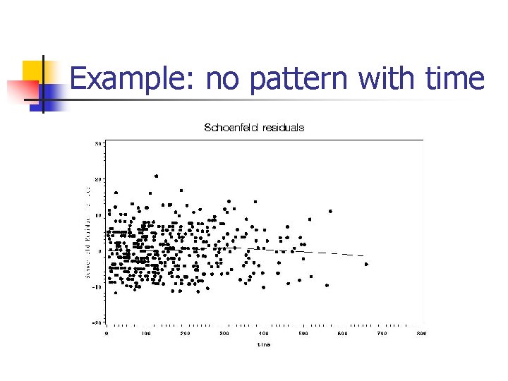
Example: no pattern with time

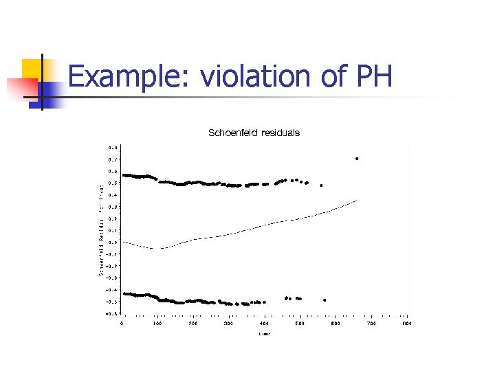
Example: violation of PH

Schoenfeld residuals In SAS: option on the output statement: Output out=outdata ressch= Covariate 1 Covariate 2 Covariate 3

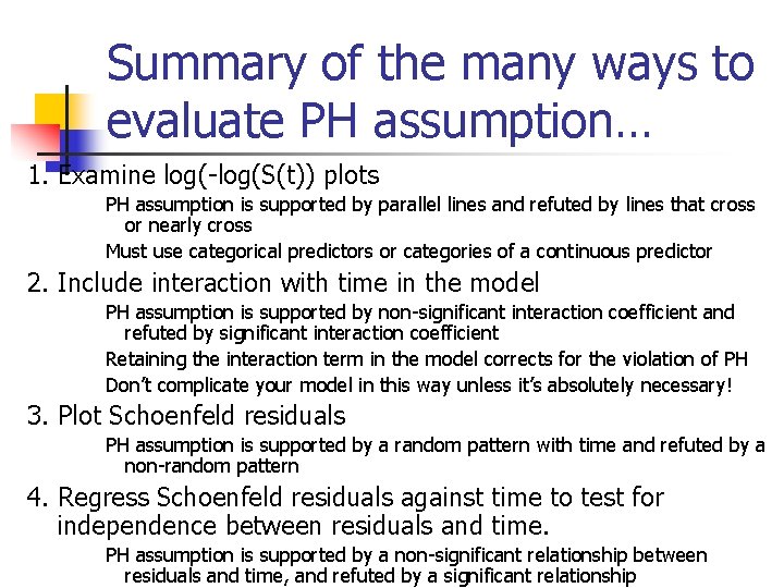
Summary of the many ways to evaluate PH assumption… 1. Examine log(-log(S(t)) plots PH assumption is supported by parallel lines and refuted by lines that cross or nearly cross Must use categorical predictors or categories of a continuous predictor 2. Include interaction with time in the model PH assumption is supported by non-significant interaction coefficient and refuted by significant interaction coefficient Retaining the interaction term in the model corrects for the violation of PH Don’t complicate your model in this way unless it’s absolutely necessary! 3. Plot Schoenfeld residuals PH assumption is supported by a random pattern with time and refuted by a non-random pattern 4. Regress Schoenfeld residuals against time to test for independence between residuals and time. PH assumption is supported by a non-significant relationship between residuals and time, and refuted by a significant relationship

4. Repeated events n Death (presumably) can only happen once, but many outcomes could happen twice… Fractures n Heart attacks n Pregnancy Etc… n

Repeated events: 1 n n Strategy 1: run a second Cox regression (among those who had a first event) starting with first event time as the origin Repeat for third, fourth, fifth, events, etc. n Problems: increasingly smaller and smaller sample sizes.

Repeated events: Strategy 2 n Treat each interval as a distinct observation, such that someone who had 3 events, for example, gives 3 observations to the dataset n Major problem: dependence between the same individual

Strategy 3 n n Stratify by individual (“fixed effects partial likelihood”) In PROC PHREG: strata id; n n Problems: does not work well with RCT data requires that most individuals have at least 2 events Can only estimate coefficients for those covariates that vary across successive spells for each individual; this excludes constant personal characteristics such as age, education, gender, ethnicity, genotype

5. Competing Risks

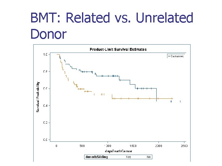
BMT: Related vs. Unrelated Donor

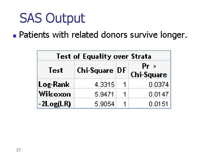
SAS Output n Patients with related donors survive longer. 37

Related/Unrelated Donor is significant. n Can you say definitively to a patient: n n 38 If you find a related donor, you will have longer survival time. What variables could be confounders?

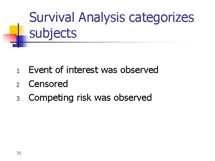
Survival Analysis categorizes subjects 1 2 3 39 Event of interest was observed Censored Competing risk was observed

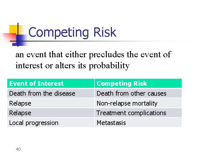
Competing Risk • an event that either precludes the event of interest or alters its probability Event of Interest Competing Risk Death from the disease Death from other causes Relapse Non-relapse mortality Relapse Treatment complications Local progression Metastasis 40

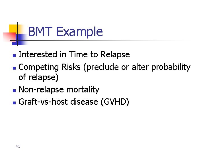
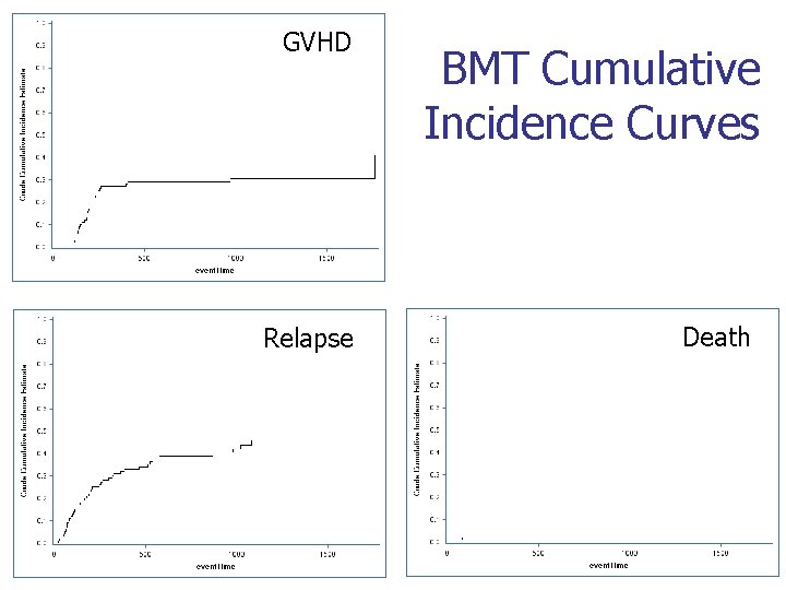
BMT Example Interested in Time to Relapse n Competing Risks (preclude or alter probability of relapse) n Non-relapse mortality n Graft-vs-host disease (GVHD) n 41

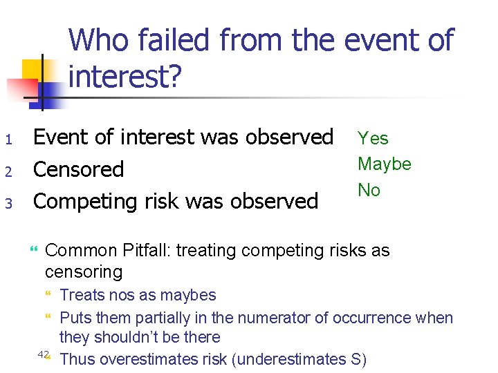
Who failed from the event of interest? 1 2 3 Event of interest was observed Censored Competing risk was observed Yes Maybe No Common Pitfall: treating competing risks as censoring 42 Treats nos as maybes Puts them partially in the numerator of occurrence when they shouldn’t be there Thus overestimates risk (underestimates S)

What to do instead KM estimate of event free survival (EFS) n Cumulative Incidence Analysis n 43

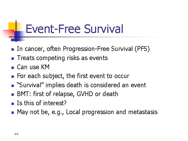
Event-Free Survival n n n n In cancer, often Progression-Free Survival (PFS) Treats competing risks as events Can use KM For each subject, the first event to occur “Survival” implies death is considered an event BMT: first of relapse, GVHD or death Is this of interest? May not be, e. g. , Local progression and metastasis 44

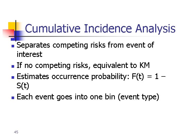
Cumulative Incidence Analysis Separates competing risks from event of interest n If no competing risks, equivalent to KM n Estimates occurrence probability: F(t) = 1 – S(t) n Each event goes into one bin (event type) n 45

GVHD Relapse BMT Cumulative Incidence Curves Death

6. Considerations when analyzing data from an RCT…

Intention-to-Treat Analysis Intention-to-treat analysis: compare outcomes according to the groups to which subjects were initially assigned, regardless of which intervention they actually received. Evaluates treatment effectiveness rather than treatment efficacy

Why intention to treat? n n Non-intention-to-treat analyses lose the benefits of randomization, as the groups may no longer be balanced with regards to factors that influence the outcome. Intention-to-treat analysis simulates “real life, ” where patients often don’t adhere perfectly to treatment or may discontinue treatment altogether.

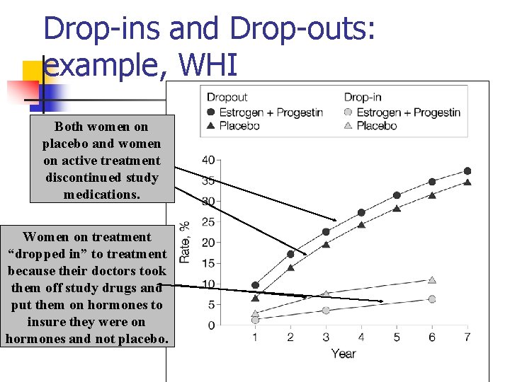
Drop-ins and Drop-outs: example, WHI Both women on placebo and women on active treatment discontinued study medications. Women on placebo “dropped Women on treatment in” to treatment because “dropped in” to treatment their regular because their doctorsput took them on hormones (dogma= them off study drugs and “hormones are good”). put them on hormones to insure they were on hormones and not placebo.

Effect of Intention to treat on the statistical analysis n Intention-to-treat analyses tend to underestimate treatment effects; increased variability due to switching “waters down” results.

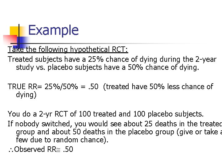
Example Take the following hypothetical RCT: Treated subjects have a 25% chance of dying during the 2 -year study vs. placebo subjects have a 50% chance of dying. TRUE RR= 25%/50% =. 50 (treated have 50% less chance of dying) You do a 2 -yr RCT of 100 treated and 100 placebo subjects. If nobody switched, you would see about 25 deaths in the treated group and about 50 deaths in the placebo group (give or take a few due to random chance). Observed RR . 50

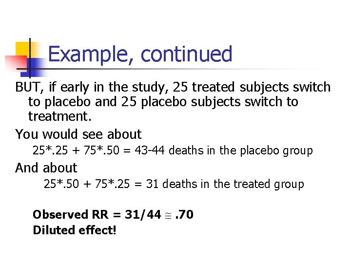
Example, continued BUT, if early in the study, 25 treated subjects switch to placebo and 25 placebo subjects switch to treatment. You would see about 25*. 25 + 75*. 50 = 43 -44 deaths in the placebo group And about 25*. 50 + 75*. 25 = 31 deaths in the treated group Observed RR = 31/44 . 70 Diluted effect!

7. Example analysis: stress fracture study • • • Women runners may have reduced levels of estrogen, which puts them at risk of bone loss and stress fractures This was a randomized trial of hormones (oral contraceptives) to prevent stress fractures in women runners Two groups: treatment and control (no placebo)

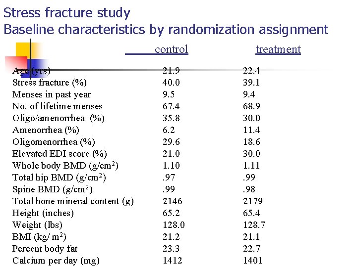
Baseline Description and Comparability of Groups n Baseline descriptors are summarized as: • • n n n means and standard deviations for continuous variables frequencies and percentages for categorical variables How good was the randomization? ; i. e. , Are the groups indeed balanced with regards to variables known to be prognostically related to the outcome? For cohort study, what factors are related to exposure, and thus might be confounders? Who is in the population?

Stress fracture study Baseline characteristics by randomization assignment control Age (yrs) Stress fracture (%) Menses in past year No. of lifetime menses Oligo/amenorrhea (%) Amenorrhea (%) Oligomenorrhea (%) Elevated EDI score (%) Whole body BMD (g/cm 2) Total hip BMD (g/cm 2) Spine BMD (g/cm 2) Total bone mineral content (g) Height (inches) Weight (lbs) BMI (kg/ m 2) Percent body fat Calcium per day (mg) 21. 9 40. 0 9. 5 67. 4 35. 8 6. 2 29. 6 21. 0 1. 10. 97. 99 2146 65. 2 128. 0 21. 2 23. 3 1412 treatment 22. 4 39. 1 9. 4 68. 9 30. 0 11. 4 18. 6 30. 0 1. 11. 99. 98 2179 65. 4 128. 7 21. 1 22. 7 1401

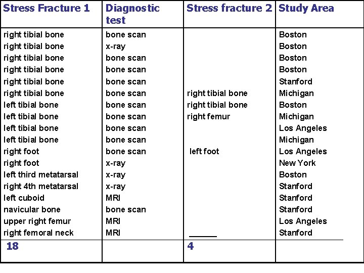
Summary of events n n Might be presented as overall incidence rates. If events are heterogeneous (as with stress fractures), tabulate results.

Stress Fracture 1 Diagnostic test right tibial bone right tibial bone left tibial bone right foot left third metatarsal right 4 th metatarsal left cuboid navicular bone upper right femur right femoral neck bone scan x-ray bone scan bone scan bone scan x-ray MRI bone scan MRI 18 Stress fracture 2 Study Area right tibial bone right femur left foot 4 Boston Stanford Michigan Boston Michigan Los Angeles New York Boston Stanford Los Angeles Stanford

Evaluation of primary hypothesis n n Intention-to-treat analysis for RCT Primary exposure-event hypothesis for cohort study, adjusted for confounding

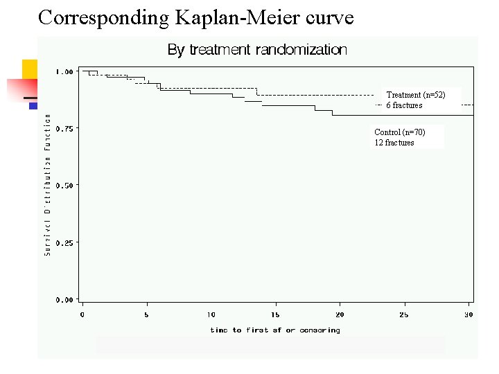
Corresponding Kaplan-Meier curve Treatment (n=52) 6 fractures Control (n=70) 12 fractures

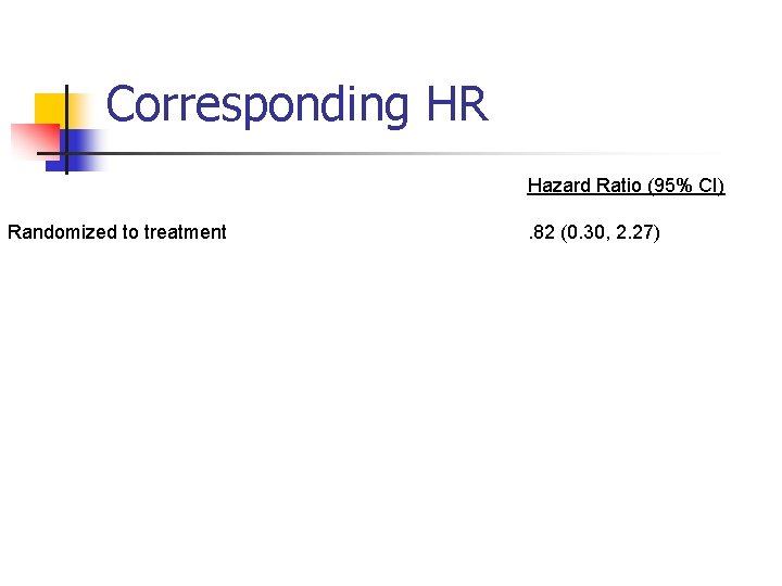
Corresponding HR Hazard Ratio (95% CI) Randomized to treatment . 82 (0. 30, 2. 27)

Secondary analyses n n For RCT: any non-intention to treat analyses For RCT and cohort: evaluate other predictors; effect modification; subgroups

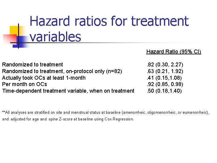
Hazard ratios for treatment variables Hazard Ratio (95% CI) Randomized to treatment, on-protocol only (n=82) Actually took OCs at least 1 -month Per month on OCs Time-dependent treatment variable, when on treatment . 82 (0. 30, 2. 27). 63 (0. 21, 1. 92). 41 (0. 15, 1. 08). 92 (0. 85, 0. 98). 50 (0. 18, 1. 40) **All analyses are stratified on site and menstrual status at baseline (amenorrheic, oligomenorrheic, or eumenorrheic), and adjusted for age and spine Z-score at baseline using Cox Regression.

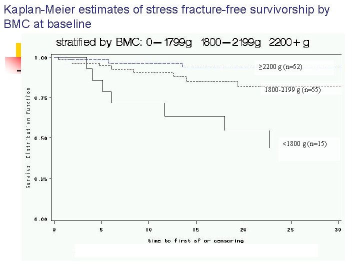
Kaplan-Meier estimates of stress fracture-free survivorship by BMC at baseline ≥ 2200 g (n=52) 1800 -2199 g (n=55) <1800 g (n=15)

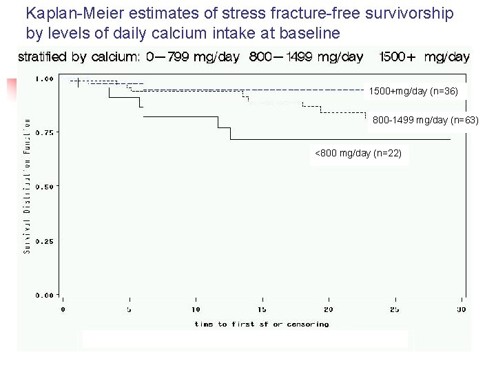
Kaplan-Meier estimates of stress fracture-free survivorship by levels of daily calcium intake at baseline 1500+mg/day (n=36) 800 -1499 mg/day (n=63) <800 mg/day (n=22)

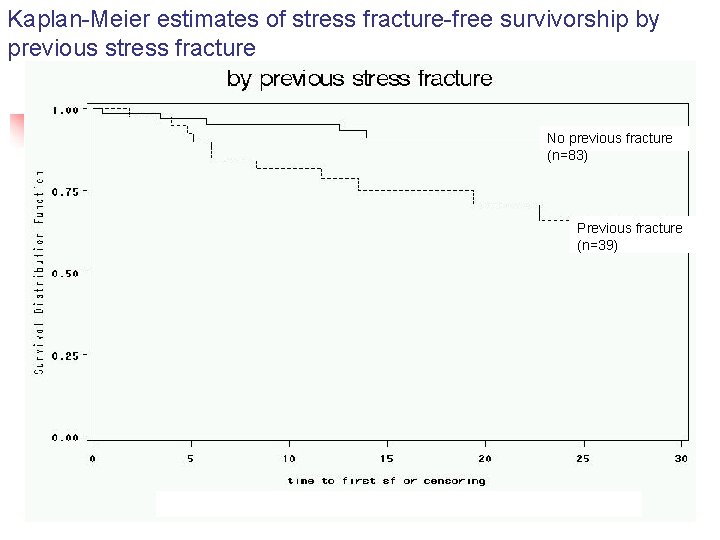
Kaplan-Meier estimates of stress fracture-free survivorship by previous stress fracture No previous fracture (n=83) Previous fracture (n=39)

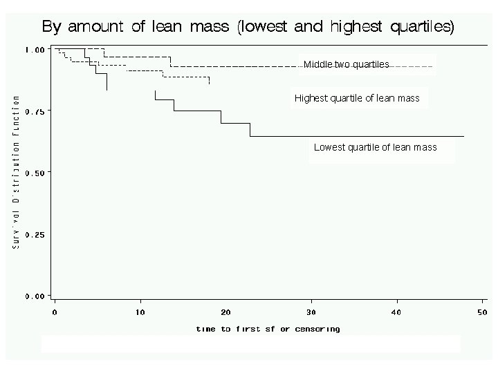
Middle two quartiles Highest quartile of lean mass Lowest quartile of lean mass

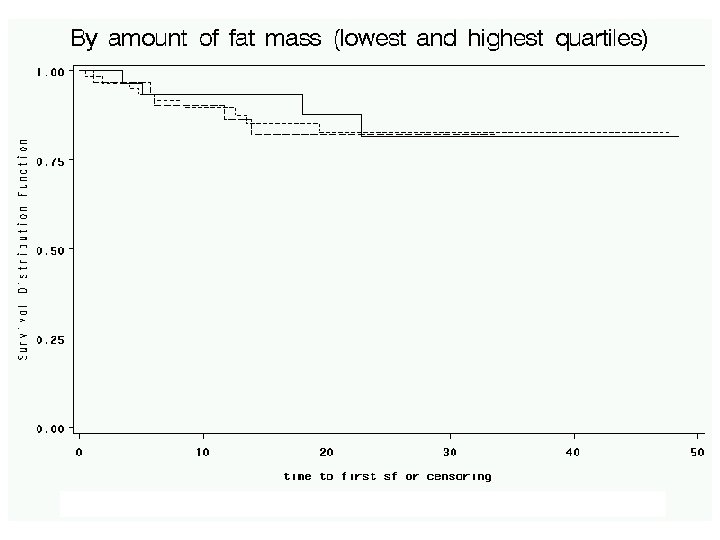
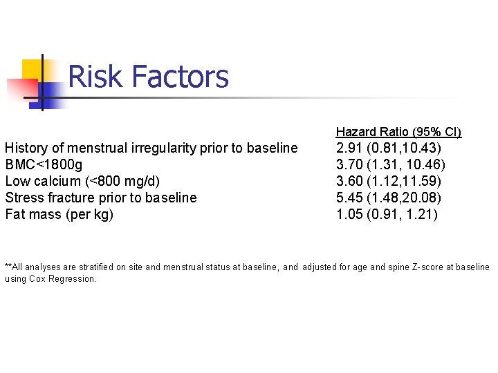
Risk Factors Hazard Ratio (95% CI) History of menstrual irregularity prior to baseline BMC<1800 g Low calcium (<800 mg/d) Stress fracture prior to baseline Fat mass (per kg) 2. 91 (0. 81, 10. 43) 3. 70 (1. 31, 10. 46) 3. 60 (1. 12, 11. 59) 5. 45 (1. 48, 20. 08) 1. 05 (0. 91, 1. 21) **All analyses are stratified on site and menstrual status at baseline, and adjusted for age and spine Z-score at baseline using Cox Regression.

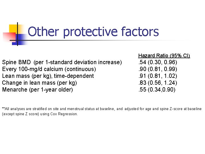
Other protective factors Hazard Ratio (95% CI) Spine BMD (per 1 -standard deviation increase) Every 100 -mg/d calcium (continuous) Lean mass (per kg), time-dependent Change in lean mass (per kg) Menarche (per 1 -year older) . 54 (0. 30, 0. 96). 90 (0. 81, 0. 99). 91 (0. 81, 1. 02). 83 (0. 56, 1. 24). 55 (0. 34, 0. 90) **All analyses are stratified on site and menstrual status at baseline, and adjusted for age and spine Z-score at baseline (except spine Z score) using Cox Regression.

References Paul Allison. Survival Analysis Using SAS Institute Inc. , Cary, NC: 2003.