Course Phylogenetic Systematics I BIOL 471 Parsimony and
 Parsimony and Parsimony Analysis Compiled by Dr. Syed")
Course: Phylogenetic Systematics I (BIOL 471) Parsimony and Parsimony Analysis Compiled by Dr. Syed Abdullah Gilani From Phylogenetics: Theory and Practice of Phylogenetic Systematics, Wiley and Lieberman, 2011, 2 nd Edition, Wiley-Blackwell, Singapore

Definition of parsimony • In English, parsimony concerns money: extreme stinginess, extreme care in spending money, reluctance to spend money unnecessarily. • The principle of parsimony is a methodological principle that posits simpler explanations of data relative to hypotheses are to be preferred over more complex explanations. • The role of parsimony was to minimize the number of ad hoc explanations embedded in the preferred hypothesis in the form of hypotheses of homoplasy (i. e. , independent evolution).

Development of parsimony method • Willi Hennig 1950 – ”Assumes that the tree that gives the fewest number of character state changes along the branches of a tree gives the best estimate of phylogeny of the characters being examined” (Fitch 2003) • Farris 1969 – Parsimony on ordered characters (morphology) – ”Wagner trees” • Fitch 1970 -1971 – Parsimony on unordered characters (nucleotides) • Sankoff 1973 – Generalized parsimony • Felsenstein 1978 – Introduces maximum likelihood to phylogenetics, and shows that parsimony could be inconsistent (”Felsenstein zone”)

Parsimony: Basic Principles 1. Among the many possible phylogenetic trees, only one of these trees is correct. 2. Characters originate and become fixed over evolutionary time transferred genetically. 3. Those taxa that share a character state are related unless they are of independent origin. 4. Once a character appears and is fixed, it will not change. 5. Characters (data columns, transformation series) are treated as independent in any analysis. 6. The result of parsimony analysis consists of placing character states on a tree where they are thought to have originated or become fixed. 7. The tree with the fewest number of independent origins of shared characters is the preferred solution. This is the maximum parsimony principle.
 • Fitch parsimony takes all")
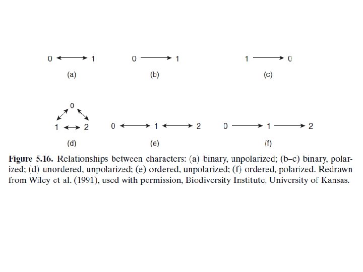
Kinds of Parsimony • Fitch parsimony (Fitch, 1971 ) • Fitch parsimony takes all characters as unordered (see Fig. 5. 16 a, d). • When three or more character states exist (Fig. 5. 16 d), a reversal from two to zero or a transformation from zero to two is counted as a single step. • This type of parsimony is commonly implemented when analyzing DNA base – pair data and multistate morphological characters. • Wagner parsimony (Farris, 1970 ) • Wagner parsimony treats binary character states identically to Fitch parsimony. • However, characters with more than two states are considered ordered (Fig. 5. 16 e). Thus a transformation from two to zero is counted as two steps because the only route from two to zero is to pass through state one.
 • General parsimony")
• “ General ” parsimony (Swofford and Olsen, 1990 ) • General parsimony allows mixing of different kinds of parsimony in a single analysis following a generalized Sankoff approach. For example, Fitch parsimony might be used for some characters, Wagner parsimony for others, and a step matrix for others. “ Informed parsimony ” is a form of general parsimony.

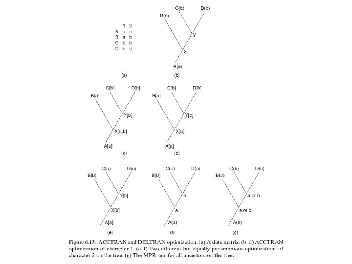
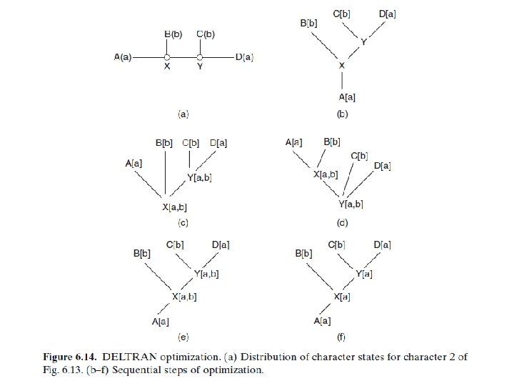
OPTIMIZING CHARACTERS ON TREES • Character optimization is an initial step in understanding the evolution of characters. It can be applied to any tree. • Character optimization is useful for the interpretation of the evolution of a particular character state. • There are two methods of interpreting character evolution, ACCTRAN and DELTRAN. • If we accelerate character transformation, then the effect is to push the time of transformation down the tree. This is commonly called ACCTRAN (accelerated transformation). • If we delay character transformation, then the effect is to push transformation up the tree. This is commonly called DELTRAN (delayed transformation).

Molecular phylogenetic tree building methods: Are mathematical and/or statistical methods for inferring the divergence order of taxa, as well as the lengths of the branches that connect them. There are many phylogenetic methods available today, each having strengths and weaknesses. Most can be classified as follows: COMPUTATIONAL METHOD Characters Distances DATA TYPE Optimality criterion Clustering algorithm PARSIMONY MAXIMUM LIKELIHOOD MINIMUM EVOLUTION UPGMA LEAST SQUARES NEIGHBOR-JOINING Based on lectures by C-B Stewart, and by Tal Pupko

Types of data used in phylogenetic inference: Character-based methods: Use the aligned characters, such as DNA or protein sequences, directly during tree inference. Taxa Species Species A B C D E Characters ATGGCTATTCTTATAGTACG ATCGCTAGTCTTATATTACA TTCACTAGACCTGTGGTCCA TTGACCAGACCTGTGGTCCG TTGACCAGTTCTCTAGTTCG Distance-based methods: Transform the sequence data into pairwise distances (dissimilarities), and then use the matrix during tree building. Species Species A B C D E A ---0. 23 0. 87 0. 73 0. 59 B 0. 20 ---0. 59 1. 12 0. 89 C 0. 50 0. 40 ---0. 17 0. 61 D 0. 45 0. 55 0. 15 ---0. 31 E 0. 40 0. 50 0. 40 0. 25 ---- Example 2: Kimura 2 -parameter distance (estimate of the true number of substitutions between taxa) Example 1: Uncorrected “p” distance (=observed percent sequence difference)

Computational methods for finding optimal trees: Exact algorithms: "Guarantee" to find the optimal or "best" tree for the method of choice. Two types used in tree building: Exhaustive search: Evaluates all possible unrooted trees, choosing the one with the best score for the method. Branch-and-bound search: Eliminates the parts of the search tree that only contain suboptimal solutions. Heuristic algorithms: Approximate or “quick-and-dirty” methods that attempt to find the optimal tree for the method of choice, but cannot guarantee to do so. Heuristic searches often operate by “hill-climbing” methods.

Exact searches become increasingly difficult, and eventually impossible, as the number of taxa increases: A B C A C B D D E A B C D F E (2 N - 5)!! = # unrooted trees for N taxa Based on lectures by C-B Stewart, and by Tal Pupko

Parsimony methods: Optimality criterion: The ‘most-parsimonious’ tree is the one that requires the fewest number of evolutionary events (e. g. , nucleotide substitutions, amino acid replacements) to explain the sequences. Advantages: • Are simple, intuitive, and logical (many possible by ‘pencil-and-paper’). • Can be used on molecular and non-molecular (e. g. , morphological) data. • Can tease apart types of similarity (shared-derived, shared-ancestral, homoplasy) • Can be used for character (can infer the exact substitutions) and rate analysis. • Can be used to infer the sequences of the extinct (hypothetical) ancestors. Disadvantages: • Are simple, intuitive, and logical (derived from “Medieval logic”, not statistics!) • Can be fooled by high levels of homoplasy (‘same’ events). • Can become positively misleading in the “Felsenstein Zone”:

How to Construct Parsimony Tree 1. Draw the three possible phylogenies for the species. 2. Tabulate the molecular data for the species. 3. Focus on site 1 in the DNA sequence. In the tree on the left. Identify and label a single base-change event. 4. Continuing the comparison of bases at sites 2, 3, and 4 reveals that each of the three trees requires a total of five additional base-change events. 5. To identify the most parsimonious tree, sum up all of the base change events noted in steps 3 and 4. 6. Conclusion: first tree is the most parsimonous.

1. Draw the three possible phylogenies for the species.

Tabulate the molecular data for the species

Focus on site 1 in the DNA sequence. In the tree on the left. Identify and label a single base-change event. Continuing the comparison of bases at sites 2, 3, and 4 reveals that each of the three trees requires a total of five additional base-change events.

sum up all of the base change events noted in steps 3 and 4.
 suggested that a useful measure of support")
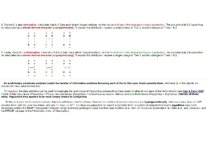
EVALUATING SUPPORT • Bremer Support. Bremer (1988) suggested that a useful measure of support for a particular clade might be the difference in the length of a tree where it appeared as a monophyletic group and the length of the tree where it did not. • Jackknife and Bootstrap.

Example II of Parsimony Analysis • For four taxa, three hypotheses of cladistic relationships can be diagrammed

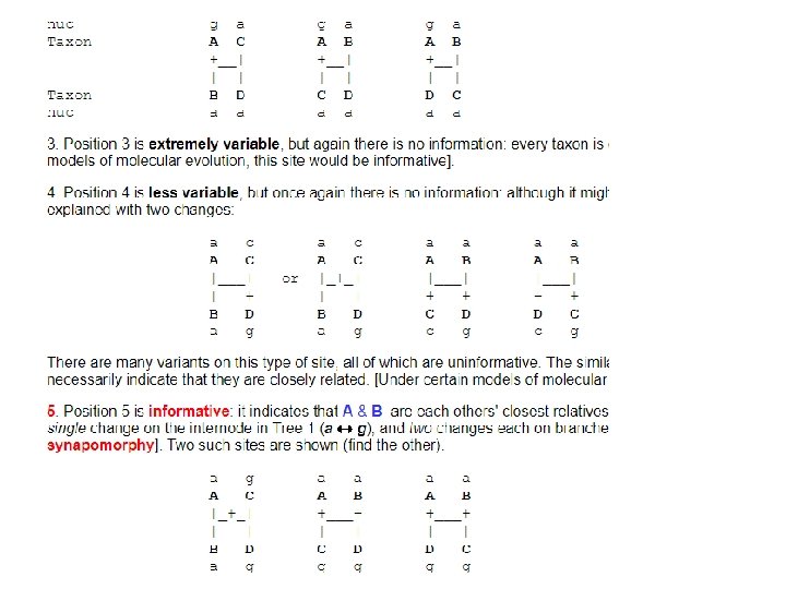
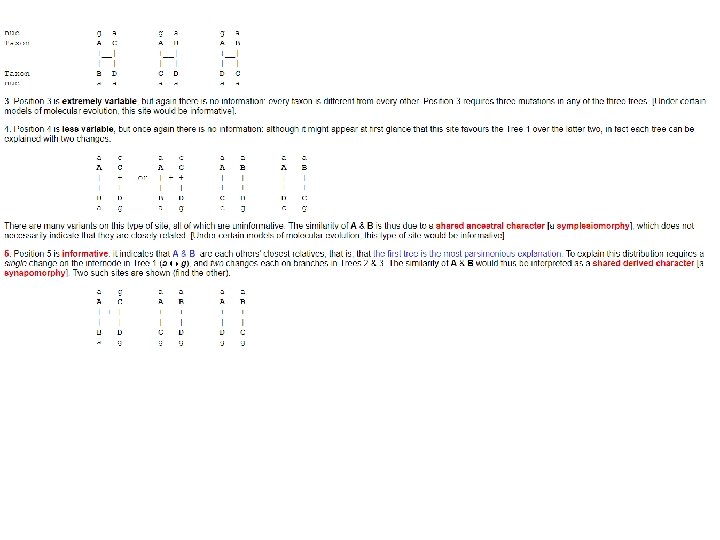
• Two kinds of nucleotide positions can be distinguished, informative and uninformative. • Informative positions are those that give information about evolutionary relationships among taxa; uninformative sites don't. • In four-taxon problem, an informative position will indicate that one of the three hypotheses is the simplest (most parsimonious) explanation of the mutational pattern implied by the data, that is, that it requires fewest mutational changes.

What is the information content of each of the seven numbered positions? 1. Position 1 is invariant: it gives no information about relationships among these taxa. The majority of sites are like this. 2. Position 2 is variable, but still gives no information: it indicates only that A is different from the other three taxa, or, put another way, that B, C, & D are similar but not that they are closely related The unique change in A at this position is therefore an autoapomorphy [a change unique to one taxon under study]. Position 2 can be explained by a single mutational change in any of the three trees. In the diagrams below, '+' indicates a change from 'a' [in B C & D] to 'g' on the branch leading to taxon A: g. [The same would be true if any one of the other three taxa were uniquely variable at this site. ] Most variable sites are of this type: five are shown in the figure above (find them)

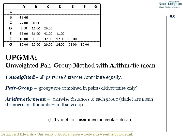
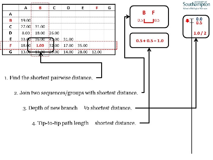
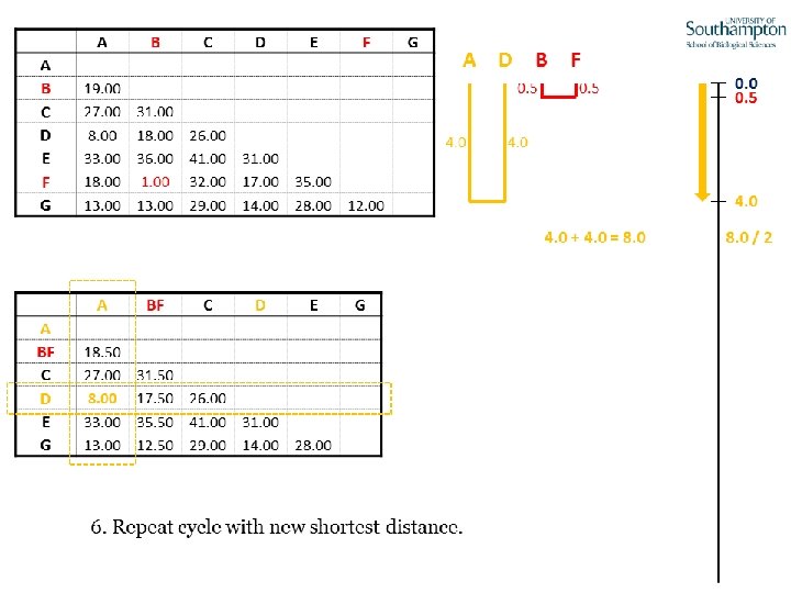
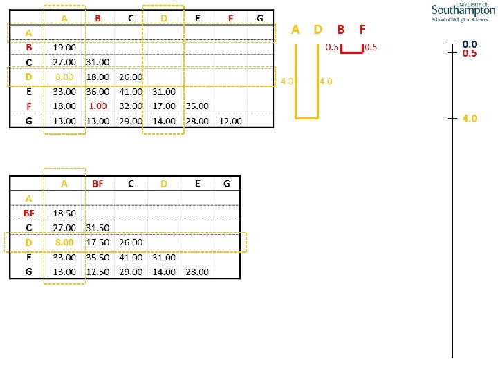
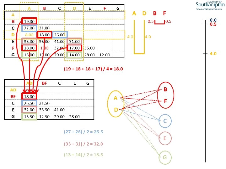
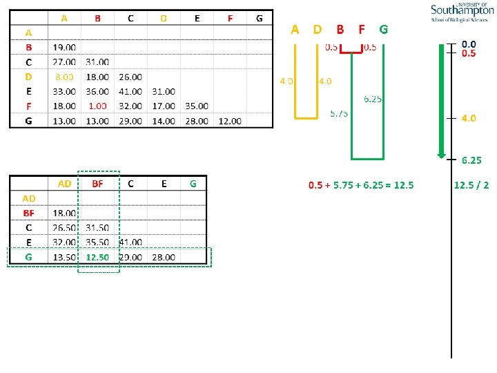
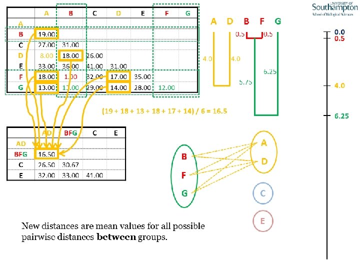
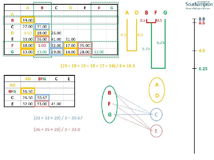
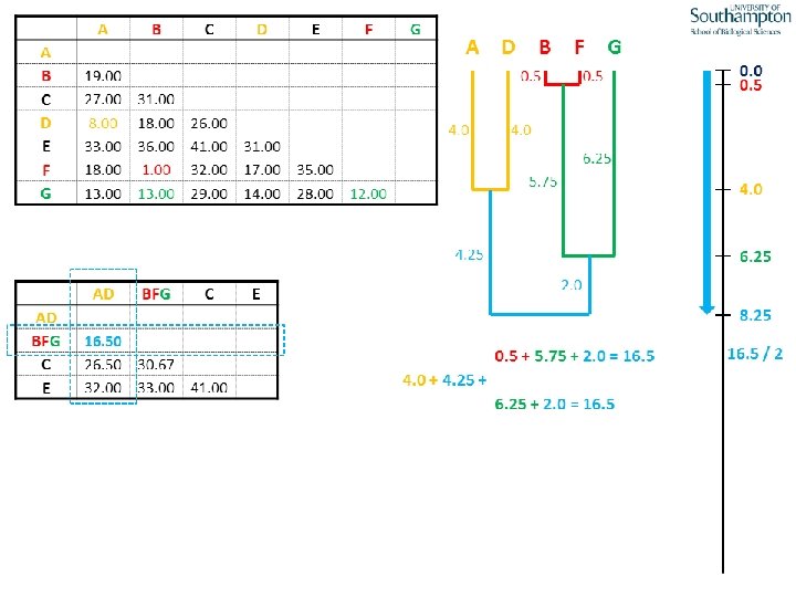
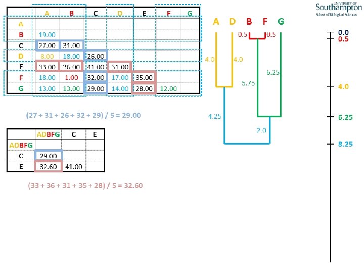
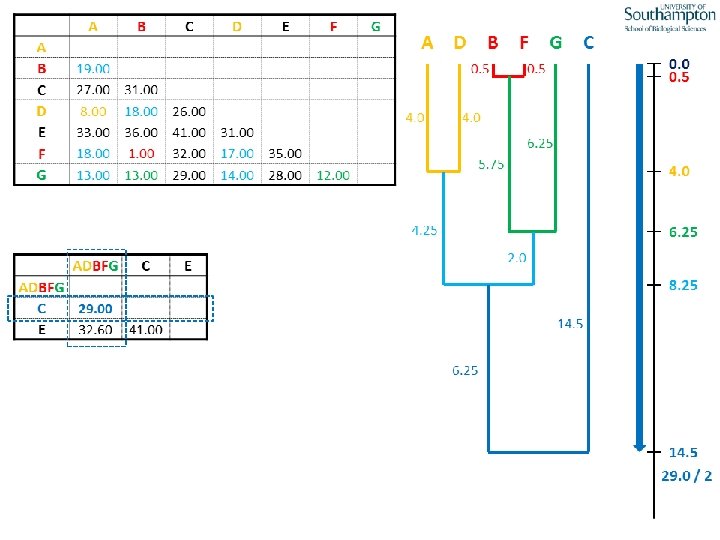
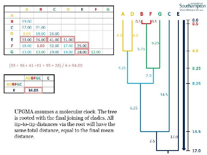
UPGMA • Example is from Dr. Richard Edwards from University of Southamptom.


References • Phylogenetics: Theory and Practice of Phylogenetic Systematics, Wiley and Lieberman, 2011, 2 nd Edition, Wiley. Blackwell, Singapore • Based on lectures by C-B Stewart, and by Tal Pupko • http: //www. cs. tau. ac. il/~bchor/CG 05/CG 7 -trees. ppt • http: //www. slimsuite. unsw. edu. au/teaching/upgma/
- Slides: 42