Course Introduction Probability Statistics and Quality Loss HW1

Course Introduction Probability, Statistics and Quality Loss HW#1 Presentations MIT

Background • SDM split-summer format – Heavily front-loaded – Systems perspective – Concern with scaling • Product development track, CIPD – Place in wider context of product realization • Joint 16 (Aero/Astro) and 2 (Mech E) MIT

Course Learning Objectives § § § § Formulate measures of performance Synthesize and select design concepts Identify noise factors Estimate the robustness Reduce the effects of noise Select rational tolerances Understand the context of RD in the end-to-end business process of product realization. MIT

Instructors • • • Dan Frey, Aero/Astro Don Clausing, Xerox Fellow Joe Saleh, TA Skip Crevelling, Guest from RIT Dave Miller, Guest from MIT Aero/Astro Others. . . MIT

Primary Text Phadke, Madhav S. , Quality Engineering Using Robust Design. Prentice Hall, 1989. MIT

Computer Hardware & Software • Required – Access to a PC running Windows 95 or NT – Office 95 or later – Reasonable proficiency with Excel • Provided – Math. Cad 7 Professional (for duration of course only) MIT

Learning Approach • Constructivism (Jean Piaget) – Knowledge is not simply transmitted – Knowledge is actively constructed in the mind of the learner (critical thought is required) • Constructionism (Seymour Papert) – People learn with particular effectiveness when they are engaged in building things, writing software, etc. – http: //el. www. media. mit. edu/groups/el/ MIT

Format of a Typical Session • Lecture • • Well, almost Reading assignment Quiz Labs, case discussions, design projects Homework MIT

Grading • Breakdown – 40% Term project – 30% Final exam – 20% Homework (~15 assignments) – 10% Quizzes (~15 quizzes) • No curve anticipated MIT

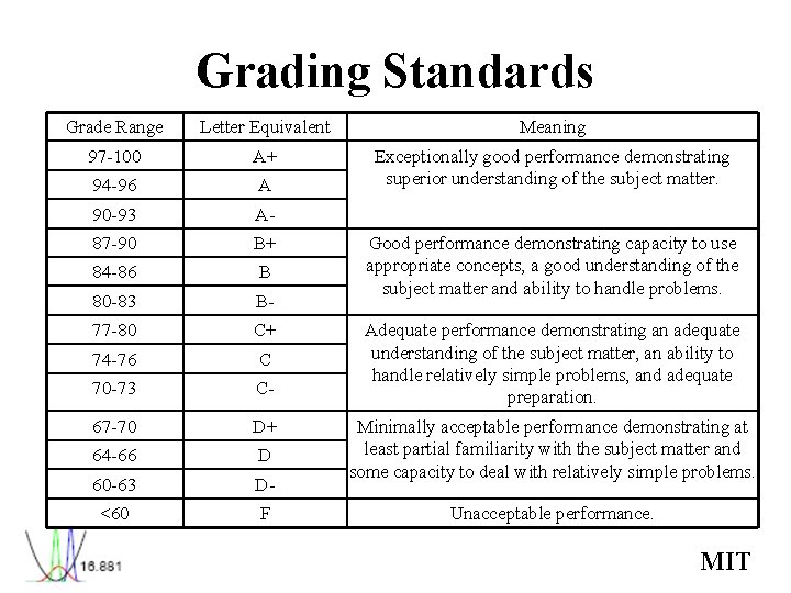
Grading Standards Grade Range Letter Equivalent Meaning 97 -100 A+ 94 -96 A Exceptionally good performance demonstrating superior understanding of the subject matter. 90 -93 A- 87 -90 B+ 84 -86 B 80 -83 B- 77 -80 C+ 74 -76 C 70 -73 C- 67 -70 D+ 64 -66 D 60 -63 D- <60 F Good performance demonstrating capacity to use appropriate concepts, a good understanding of the subject matter and ability to handle problems. Adequate performance demonstrating an adequate understanding of the subject matter, an ability to handle relatively simple problems, and adequate preparation. Minimally acceptable performance demonstrating at least partial familiarity with the subject matter and some capacity to deal with relatively simple problems. Unacceptable performance. MIT

Reading Assignment • Taguchi and Clausing, “Robust Quality” • Major Points – Quality loss functions (Lecture 1) – Overall context of RD (Lecture 2) – Orthogonal array based experiments (Lecture 3) – Two-step optimization for robustness • Questions? MIT

Learning Objectives • Review some fundamentals of probability and statistics • Introduce the quality loss function • Tie the two together • Discuss in the context of engineering problems MIT

Probability Definitions • Sample space -List all possible outcomes of an experiment – Finest grained – Mutually exclusive – Collectively exhaustive • Event -A collection of points or areas in the sample space MIT

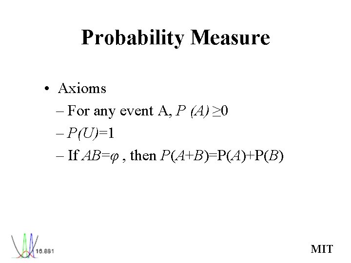
Probability Measure • Axioms – For any event A, P (A) ≥ 0 – P(U)=1 – If AB=φ , then P(A+B)=P(A)+P(B) MIT

Discrete Random Variables • A random variable that can assume any of a set of discrete values • Probability mass function – px(xo) = probability that the random variable x will take the value xo – Let’s build a pmf for one of the examples • Event probabilities computed by summation MIT

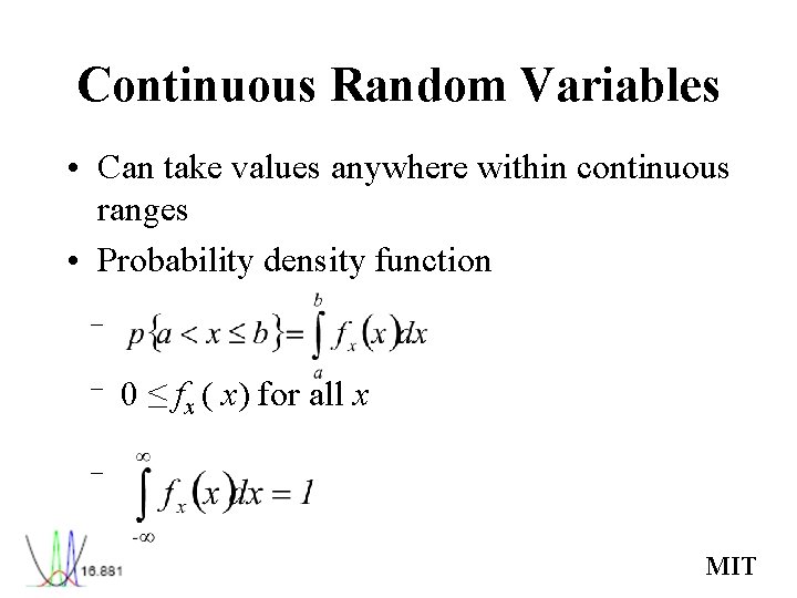
Continuous Random Variables • Can take values anywhere within continuous ranges • Probability density function – – 0 ≤ fx ( x) for all x – MIT

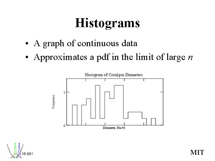
Histograms • A graph of continuous data • Approximates a pdf in the limit of large n MIT

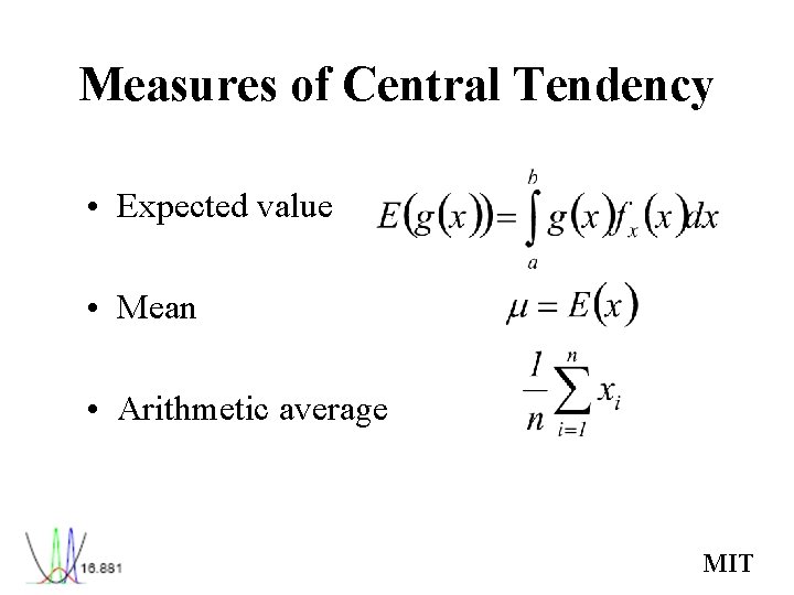
Measures of Central Tendency • Expected value • Mean • Arithmetic average MIT

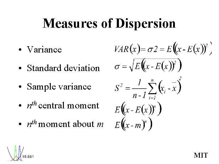
Measures of Dispersion • Variance • Standard deviation • Sample variance • nth central moment • nth moment about m MIT

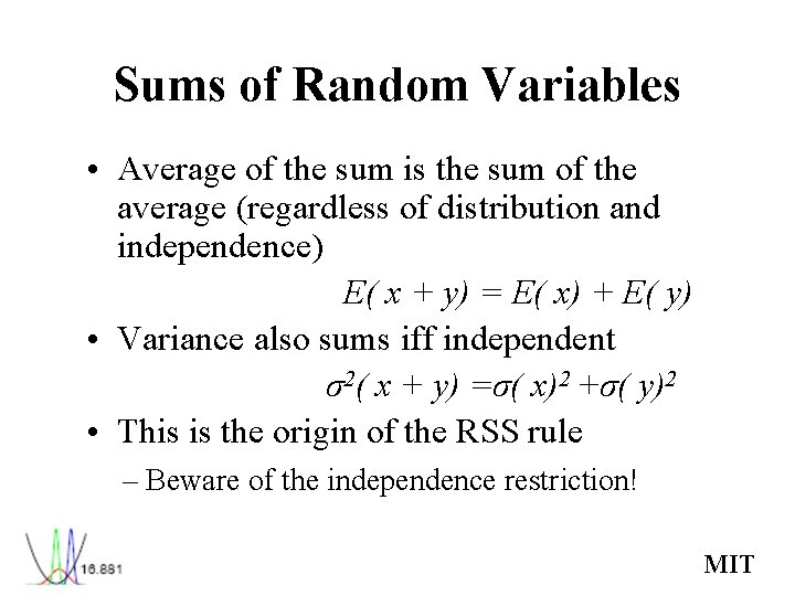
Sums of Random Variables • Average of the sum is the sum of the average (regardless of distribution and independence) E( x + y) = E( x) + E( y) • Variance also sums iff independent σ2( x + y) =σ( x)2 +σ( y)2 • This is the origin of the RSS rule – Beware of the independence restriction! MIT

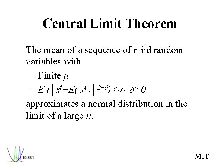
Central Limit Theorem The mean of a sequence of n iid random variables with – Finite μ – E (│xi−E( xi )│2+δ)<∞ δ>0 approximates a normal distribution in the limit of a large n. MIT

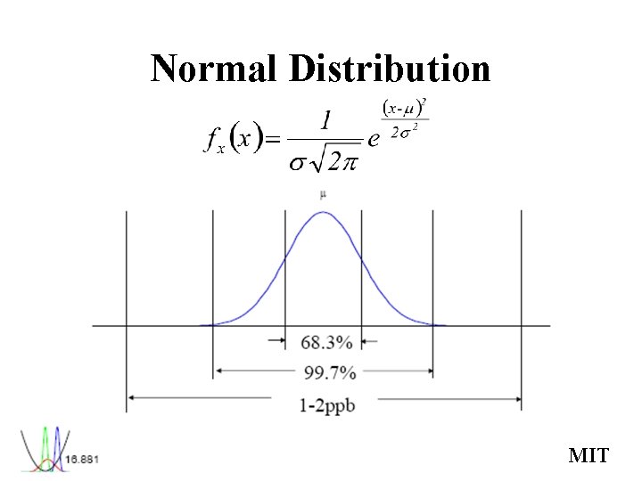
Normal Distribution MIT

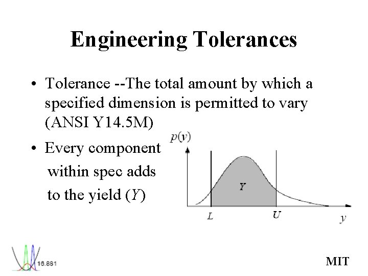
Engineering Tolerances • Tolerance --The total amount by which a specified dimension is permitted to vary (ANSI Y 14. 5 M) • Every component within spec adds to the yield (Y) MIT

Crankshafts • What does a crankshaft do? • How would you define the tolerances? • How does variation affect performance? MIT

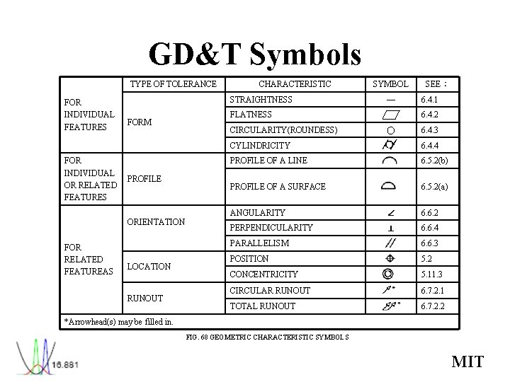
GD&T Symbols TYPE OF TOLERANCE FOR INDIVIDUAL FEATURES FOR INDIVIDUAL OR RELATED FEATURES STRAIGHTNESS FORM PROFILE ORIENTATION FOR RELATED FEATUREAS CHARACTERISTIC LOCATION RUNOUT SYMBOL ― FLATNESS CIRCULARITY(ROUNDESS) SEE： 6. 4. 1 6. 4. 2 ○ 6. 4. 3 CYLINDRICITY 6. 4. 4 PROFILE OF A LINE 6. 5. 2(b) PROFILE OF A SURFACE 6. 5. 2(a) ANGULARITY ∠ 6. 6. 2 PERPENDICULARITY ⊥ 6. 6. 4 PARALLELISM 6. 6. 3 POSITION 5. 2 CONCENTRICITY 5. 11. 3 CIRCULAR RUNOUT 6. 7. 2. 1 TOTAL RUNOUT 6. 7. 2. 2 *Arrowhead(s) may be filled in. FIG. 68 GEOMETRIC CHARACTERISTIC SYMBOLS MIT

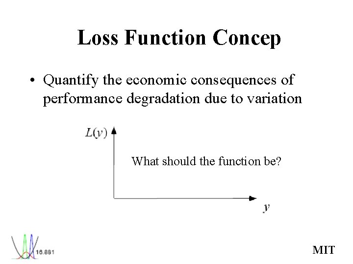
Loss Function Concep • Quantify the economic consequences of performance degradation due to variation What should the function be? MIT

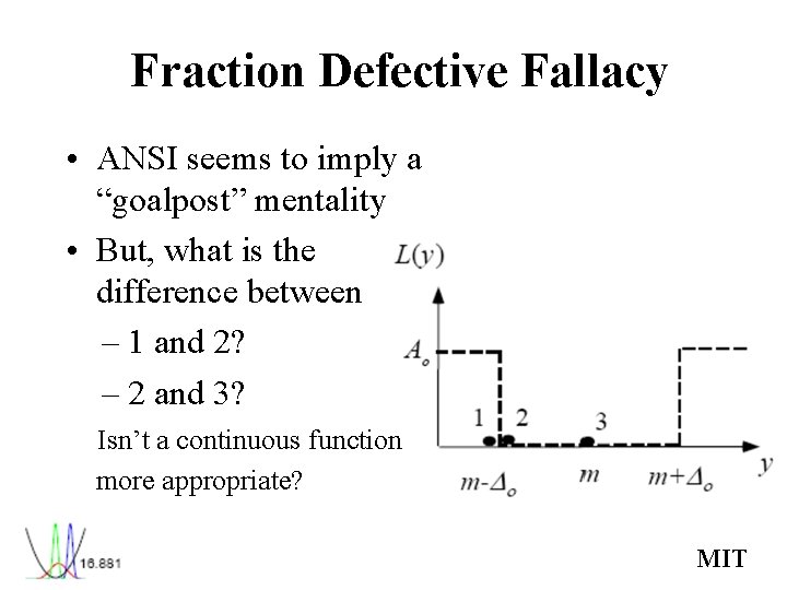
Fraction Defective Fallacy • ANSI seems to imply a “goalpost” mentality • But, what is the difference between – 1 and 2? – 2 and 3? Isn’t a continuous function more appropriate? MIT

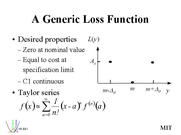
A Generic Loss Function • Desired properties – Zero at nominal value – Equal to cost at specification limit – C 1 continuous • Taylor series MIT

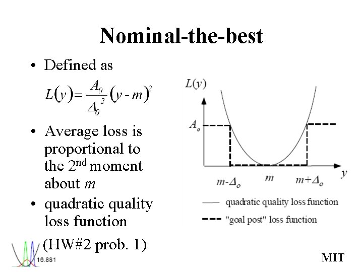
Nominal-the-best • Defined as • Average loss is proportional to the 2 nd moment about m • quadratic quality loss function (HW#2 prob. 1) MIT

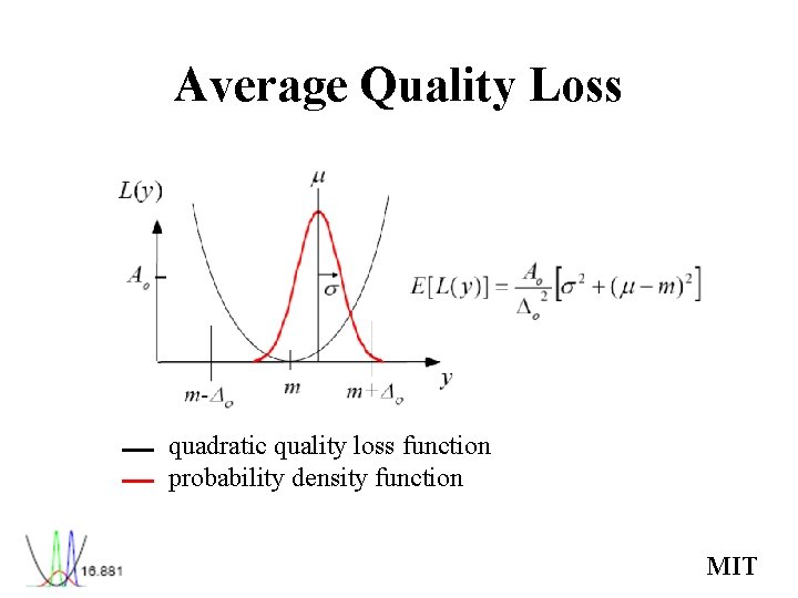
Average Quality Loss quadratic quality loss function probability density function MIT

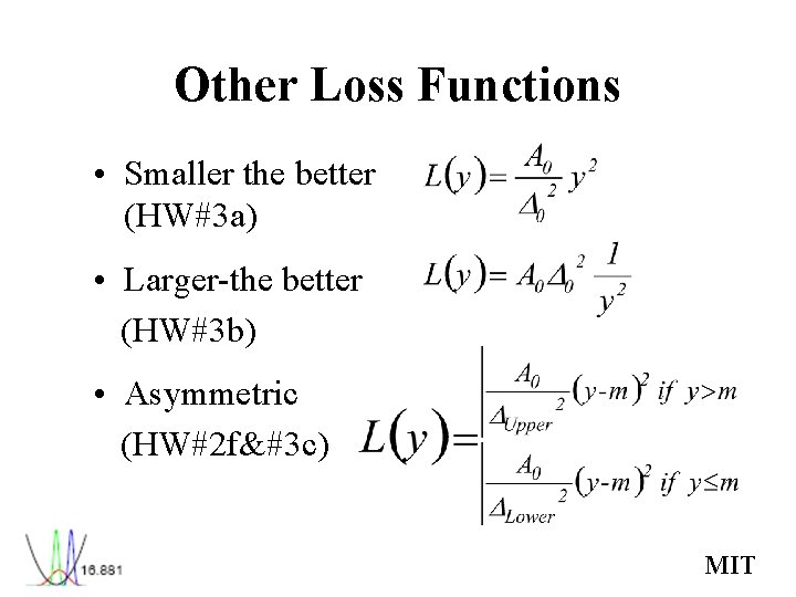
Other Loss Functions • Smaller the better (HW#3 a) • Larger-the better (HW#3 b) • Asymmetric (HW#2 f&#3 c) MIT

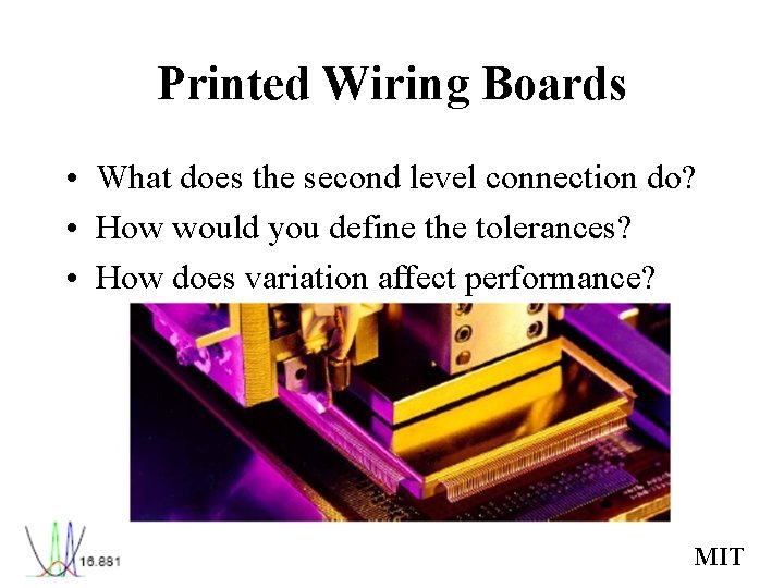
Printed Wiring Boards • What does the second level connection do? • How would you define the tolerances? • How does variation affect performance? MIT

Next Steps • Load Mathcad (if you wish) • Optional Mathcad tutoring session – 1 hour Session • Complete Homework #2 • Read Phadke ch. 1 & 2 and session #2 notes • Next lecture – Don Clausing, Context of RD in PD MIT