COURSE 4 4 OPTIMIZATION PROGRAMMES 1 OPTIMIZATION PROGRAMMES

- COURSE 4. 4 OPTIMIZATION PROGRAMMES 1

OPTIMIZATION PROGRAMMES Peter Kelderman UNESCO-IHE Institute for Water Education Online Module Water Quality Assessment

A general view of information The “Data-rich but Information-poor” syndrome in water quality monitoring (Ward, R. C. , J. C. Loftis and G. B. Mc. Bride, 1986) “Research reports are lying in dusty drawers of policy makers or elsewhere and never used” (Boogerd, A. , P. Groenewegen and M. Hisschemöller, 1997) 3

Refresher Course Rwanda, 22 -26 October 2012 4

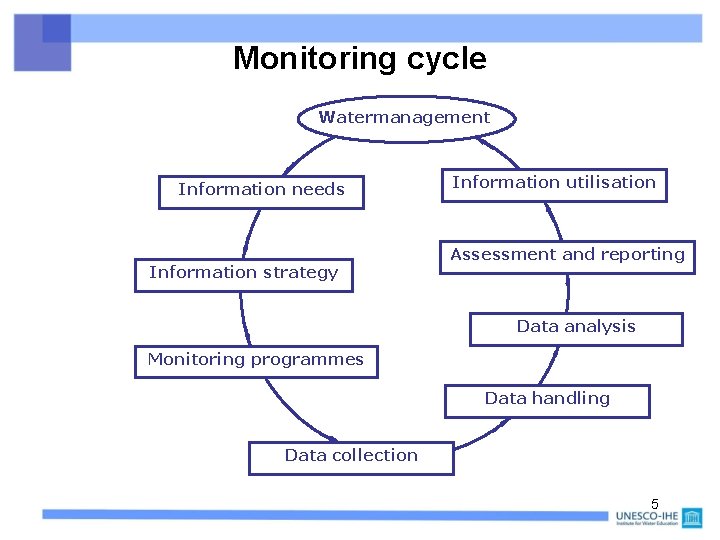
Monitoring cycle Watermanagement Information needs Information strategy Information utilisation Assessment and reporting Data analysis Monitoring programmes Data handling Data collection 5

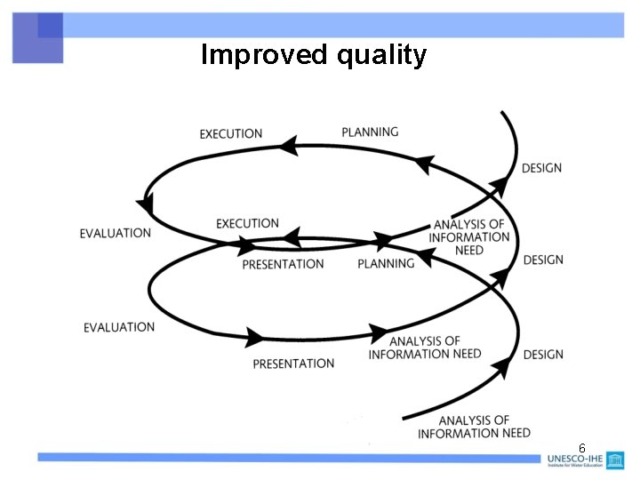
Improved quality 6

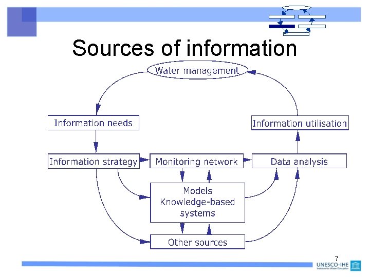
Sources of information 7

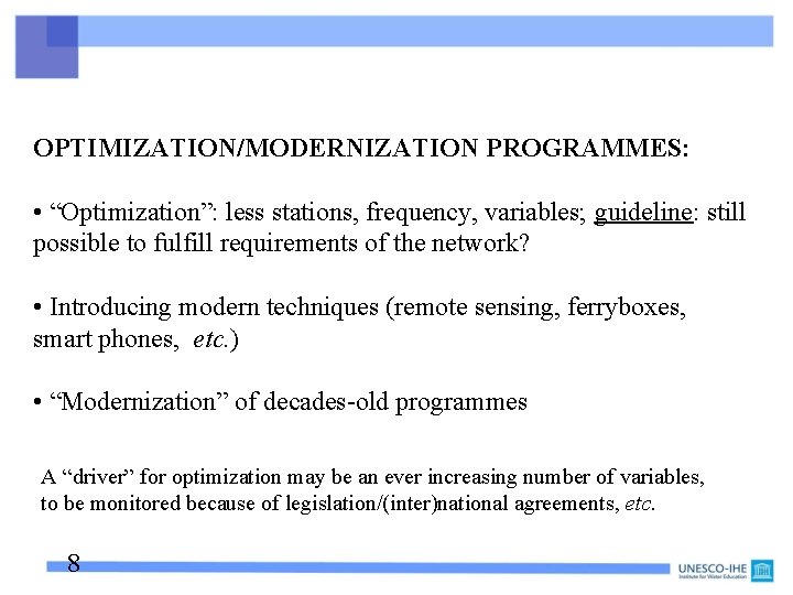
OPTIMIZATION/MODERNIZATION PROGRAMMES: • “Optimization”: less stations, frequency, variables; guideline: still possible to fulfill requirements of the network? • Introducing modern techniques (remote sensing, ferryboxes, smart phones, etc. ) • “Modernization” of decades-old programmes A “driver” for optimization may be an ever increasing number of variables, to be monitored because of legislation/(inter)national agreements, etc. 8

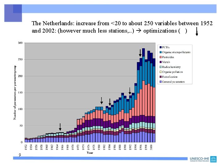
The Netherlands: increase from <20 to about 250 variables between 1952 and 2002: (however much less stations, . . ) optimizations ( ) 9

OPTIMIZATION PROGRAMMES Criteria for optimization of monitoring networks: • Optimized network still gives reliable overview of the water quality in the area? Network still according to (inter)national agreements and legislation? • Measuring frequency? according to “relevant margins” • Trends can still be detected? (e. g. over 5 years) • With two stations A and B: leave out A or B, in case of certain minimum level of correlation between A and B; the same holds for correlation between two variables (see before: NH 4 -N vs. Ntot. ) 10

Example: It can be decided to leave out station B if for > 90% of the variables, the correlation coefficient r between A and B is larger than 0. 8 (= recommendation in the Netherlands; “governmental waters”) 11

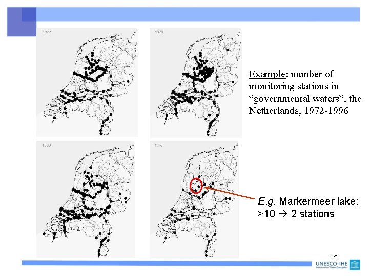
Example: number of monitoring stations in “governmental waters”, the Netherlands, 1972 -1996 E. g. Markermeer lake: >10 2 stations 12

You have to keep in mind factors such as: • Data dependence between stations (e. g. in rivers); “autocorrelation” • Seasonal trends? Often have to be “filtered out” using tests: Kruskal-Wallis or ANOVA • Using the relevant margins, monitoring frequencies may be unrealistically high make compromises (see EU-WFD) • How to deal with “outliers” in a data set? (Dixon Q test? + 3 or 4 standard deviations away from average? ) 13

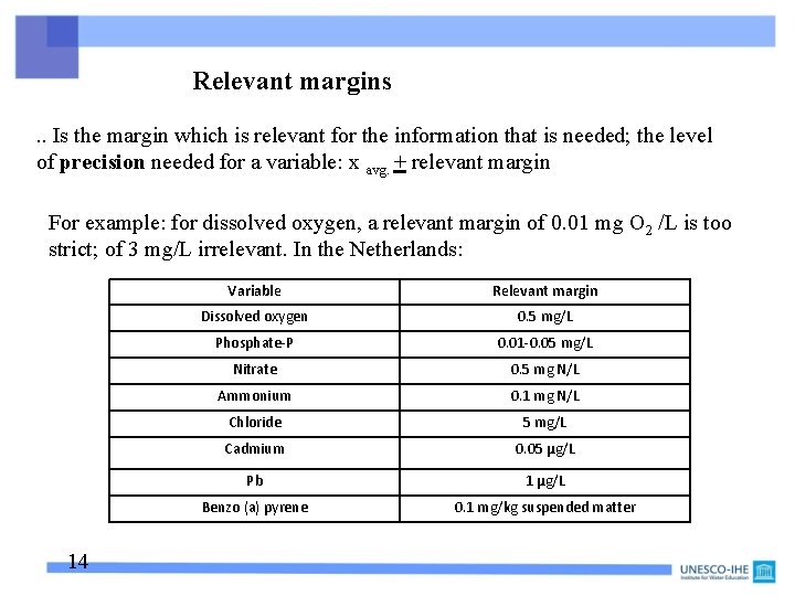
Relevant margins. . Is the margin which is relevant for the information that is needed; the level of precision needed for a variable: x avg. + relevant margin For example: for dissolved oxygen, a relevant margin of 0. 01 mg O 2 /L is too strict; of 3 mg/L irrelevant. In the Netherlands: 14 Variable Relevant margin Dissolved oxygen 0. 5 mg/L Phosphate-P 0. 01 -0. 05 mg/L Nitrate 0. 5 mg N/L Ammonium 0. 1 mg N/L Chloride 5 mg/L Cadmium 0. 05 µg/L Pb 1 µg/L Benzo (a) pyrene 0. 1 mg/kg suspended matter

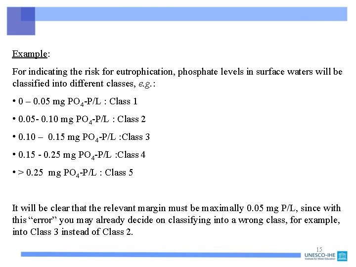
Example: For indicating the risk for eutrophication, phosphate levels in surface waters will be classified into different classes, e. g. : • 0 – 0. 05 mg PO 4 -P/L : Class 1 • 0. 05 - 0. 10 mg PO 4 -P/L : Class 2 • 0. 10 – 0. 15 mg PO 4 -P/L : Class 3 • 0. 15 - 0. 25 mg PO 4 -P/L : Class 4 • > 0. 25 mg PO 4 -P/L : Class 5 It will be clear that the relevant margin must be maximally 0. 05 mg P/L, since with this “error” you may already decide on classifying into a wrong class, for example, into Class 3 instead of Class 2. 15

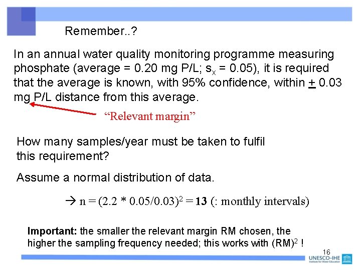
Remember. . ? In an annual water quality monitoring programme measuring phosphate (average = 0. 20 mg P/L; sx = 0. 05), it is required that the average is known, with 95% confidence, within + 0. 03 mg P/L distance from this average. “Relevant margin” How many samples/year must be taken to fulfil this requirement? Assume a normal distribution of data. n = (2. 2 * 0. 05/0. 03)2 = 13 (: monthly intervals) Important: the smaller the relevant margin RM chosen, the higher the sampling frequency needed; this works with (RM)2 ! 16

STEP-BY-STEP OPTIMIZATION OF WATER QUALITY MONITORING NETWORKS 17

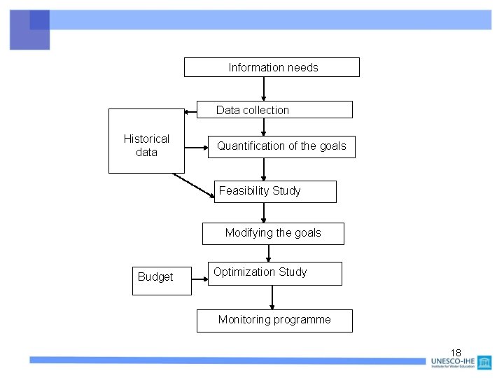
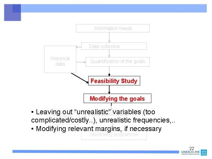
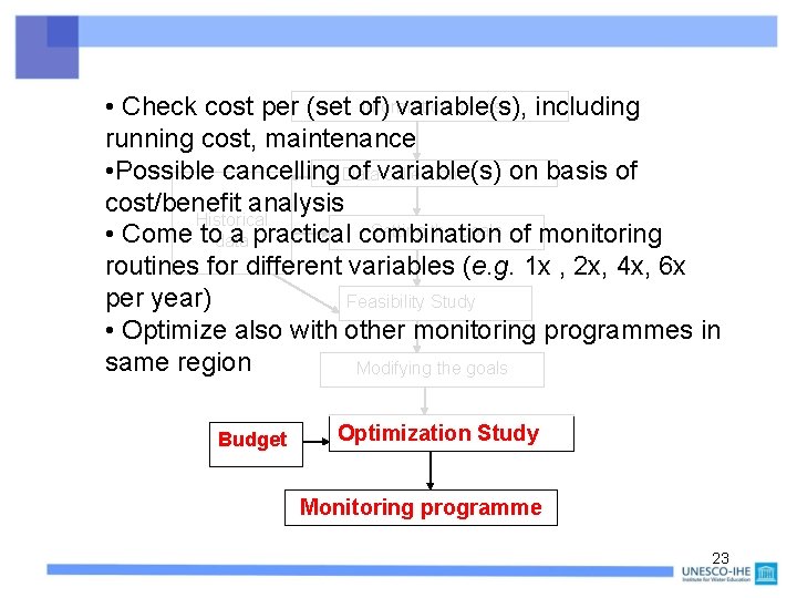
Information needs Data collection Historical data Quantification of the goals Feasibility Study Modifying the goals Budget Optimization Study Monitoring programme 18

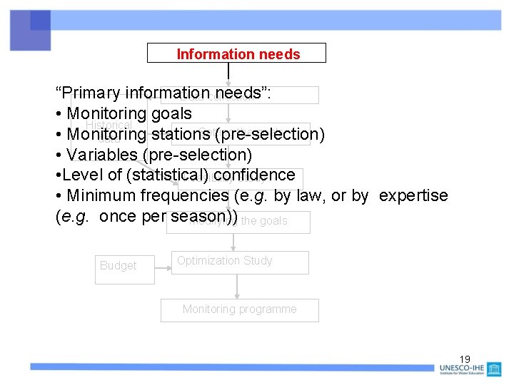
Information needs “Primary information needs”: Data collection • Monitoring goals Historical Setting the goals • Monitoring stations (pre-selection) data • Variables (pre-selection) • Level of (statistical) confidence Feasibility Study • Minimum frequencies (e. g. by law, or by expertise (e. g. once per season)) Modifying the goals Budget Optimization Study Monitoring programme 19

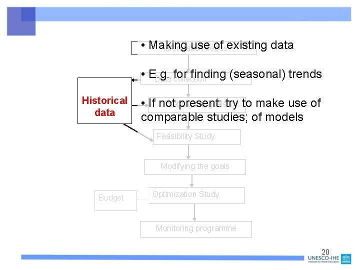
• Making useneeds of existing data Information • E. g. finding (seasonal) trends Data for collection Historical data • If not present: Setting the goalstry to make use of comparable studies; of models Feasibility Study Modifying the goals Budget Optimization Study Monitoring programme 20

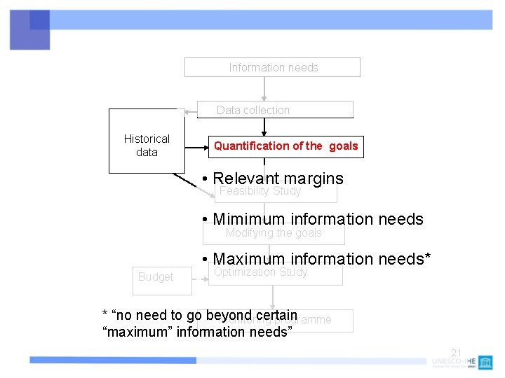
Information needs Data collection Historical data Quantification of the goals • Relevant margins Feasibility Study • Mimimum information needs Modifying the goals • Maximum information needs* Budget Optimization Study * “no need to go beyond certain Monitoring programme “maximum” information needs” 21

Information needs Data collection Historical data Quantification of the goals Feasibility Study Modifying the goals • Leaving out “unrealistic” variables (too Optimization Study Budget complicated/costly. . ), unrealistic frequencies, . . • Modifying relevant margins, if necessary Monitoring programme 22

Information needs • Check cost per (set of) variable(s), including running cost, maintenance • Possible cancelling Data of variable(s) on basis of collection cost/benefit analysis Historical Setting the goals of monitoring • Come todata a practical combination routines for different variables (e. g. 1 x , 2 x, 4 x, 6 x per year) Feasibility Study • Optimize also with other monitoring programmes in same region Modifying the goals Budget Optimization Study Monitoring programme 23

Measuring stations: • Representative for their surrounding • Not too high variability • Can give clear indication of “trends”, e. g. after sanitation Variables; “indicator variables” are most suitable; be careful with: • Variables with hardly any added values • With extreme variability in time and space (e. g. susp. solids) • With excessive cost (like organic micropollutants) 24

A WQ monitoring network is “optimal” if: • “Everywhere” and at any time, the water quality is known, with sufficient reliability • Each station is representative for a certain type of water, or area • There is no overlap in info between stations • The programme fits well with other monitoring programmes and monitoring objectives. 25

COST ASPECTS: Highest cost: sampling and analysis If cost are too high for budget: • Ask for higher budget • Reduce the number of variables, and/or frequency and/or stations (see e. g. Course 3. 9. ) • Give much attention to relatively “inexpensive” factors 26