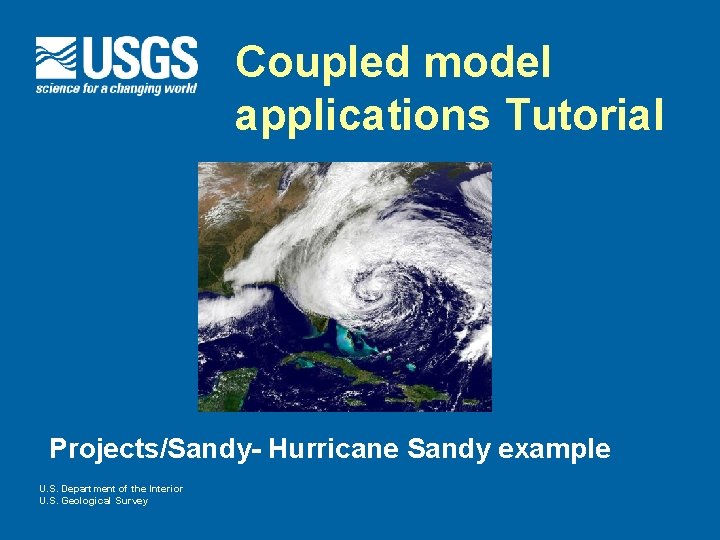
Coupled model applications Tutorial ProjectsSandy Hurricane Sandy example

Coupled model applications Tutorial Projects/Sandy- Hurricane Sandy example U. S. Department of the Interior U. S. Geological Survey

- How does the coupled modeling system work (MCT) - SCRIP interpolation - Setting up a coupled application

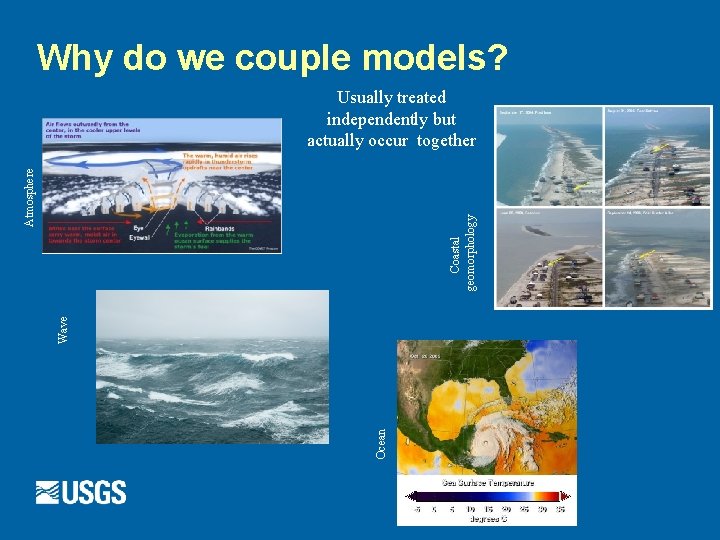
Why do we couple models? Ocean Wave Coastal geomorphology Atmosphere Usually treated independently but actually occur together

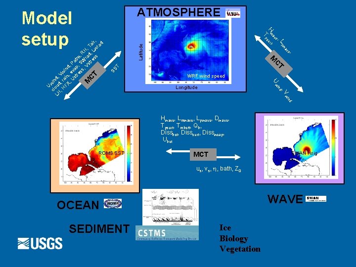
ATMOSPHERE Latitude C T WRF wind speed Uw M C SS T T , e av M r, ai rad T , H , Lw , R rad s tm es Pa , SW str , V d p in va ss, w e e V , tr d, in s in , ra , U w U oud HFX cl H, L pw , L e av , H w surf Tp Model setup , V d in Longitude nd wi Hwave, Lmwave, Lpwave, Dwave, Tpsurf, Tmbott, Qb, Dissbot, Disssurf, Disswcap, Ubot ROMS SST SWAN Hsig MCT us, vs, h, bath, Z 0 WAVE OCEAN SEDIMENT Ice Biology Vegetation

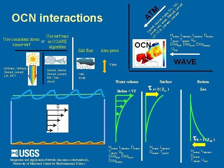
r, ai rad T , H , Lw , R rad s tm es Pa , SW str , V d p in va ss, w e e V , tr d, in s in , ra , U w U oud HFX cl H, Hwave, Lmwave, L OCN interactions Use wrf vars Use consistent stress or in COARE roms+wrf algorithm Salt flux A Atm press TM Lpwave, Dwave, Tpsurf, Tmbott, Qb, Dissbot, Disssurf, Disswcap, Ubot OCN WAVE Patm Ustress, Vstress, Swrad, Lwrad LH, HFX Uwind, Vwind Swrad, Lwrad, RH, Tair, cloud rain, evap Water column Stokes + VF Surface t s= f ( Z os ) Bottom Zoa tb = f ( Z Integration and Application Network (ian. umces. edu/symbols), University of Maryland Center for Environmental Science. Hwave, Lmwave, Dwave, Tpsurf, Qb, Dissbot, Disssurf, Disswcap, Hwave, Lpwave, Dwave, Tpsurf, ob Hwave, Lmwave, Dwave, Tmbott, Ubot )

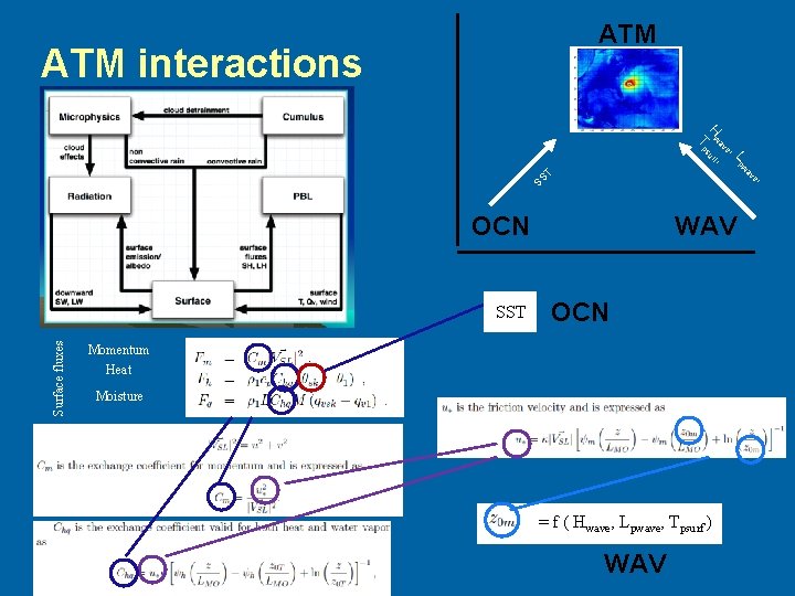
ATM interactions pw , L e av , H w surf Tp , e av T SS OCN Surface fluxes SST WAV OCN Momentum Heat Moisture = f ( Hwave, Lpwave, Tpsurf ) WAV

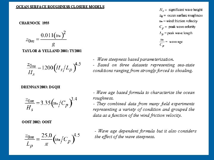
OCEAN SURFACE ROUGHNESS CLOSURE MODELS CHARNOCK 1955 TAYLOR & YELLAND 2001: TY 2001 - Wave steepness based parameterization. - Based on three datasets representing sea-state conditions ranging from strongly forced to shoaling. DRENNAN 2003: DGQH - Wave age based formula to characterize the ocean roughness. - They combined data from many field experiments representing a variety of condition and grouped the data as a function of the wind friction velocity. OOST 2002: OOST - Wave age dependent formula but it also considers the effect of the wave steepness.

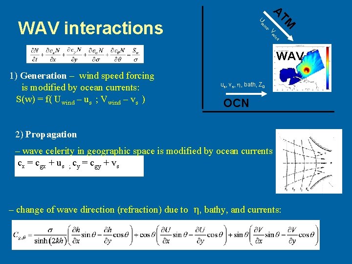
, V d in Uw WAV interactions A TM d in w WAV 1) Generation – wind speed forcing is modified by ocean currents: S(w) = f( Uwind – us ; Vwind – vs ) us, vs, h, bath, Z 0 OCN 2) Propagation – wave celerity in geographic space is modified by ocean currents cx = cgx + us ; cy = cgy + vs – change of wave direction (refraction) due to h, bathy, and currents:

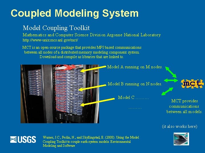
Coupled Modeling System Model Coupling Toolkit Mathematics and Computer Science Division Argonne National Laboratory http: //www-unix. mcs. anl. gov/mct/ MCT is an open-source package that provides MPI based communications between all nodes of a distributed memory modeling component system. Download and compile as libraries that are linked to. Model A running on M nodes. Model B running on N nodes. Model C ……… MCT provides communications between all models. (it also works here) Warner, J. C. , Perlin, N. , and Skyllingstad, E. (2008). Using the Model Coupling Toolkit to couple earth system models. Environmental Modeling and Software

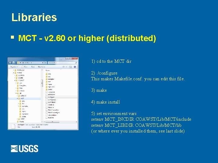
Libraries § MCT - v 2. 60 or higher (distributed) 1) cd to the MCT dir 2). /configure This makes Makefile. conf. you can edit this file. 3) make 4) make install 5) set environment vars setenv MCT_INCDIR COAWST/Lib/MCT/include setenv MCT_LIBDIR COAWST/Lib/MCT/lib (or where ever you installed them, see last slide)

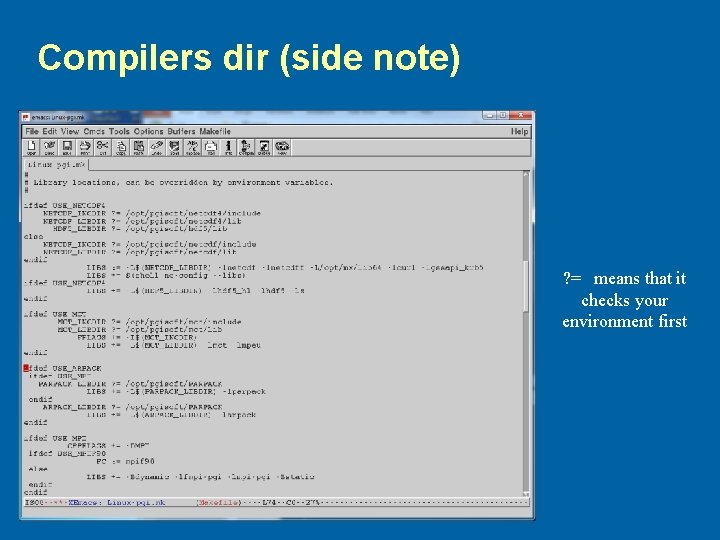
Compilers dir (side note) ? = means that it checks your environment first

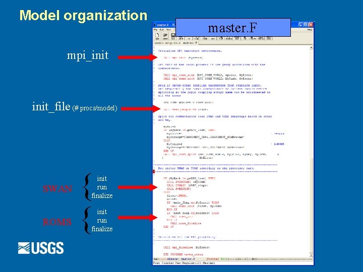
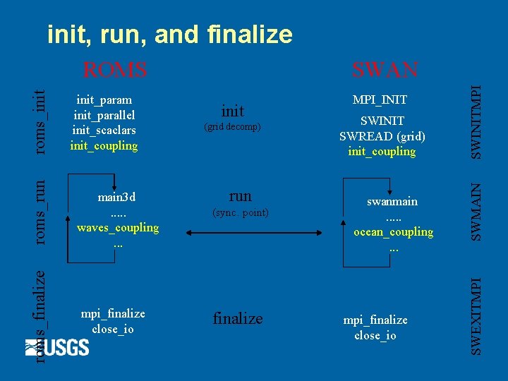
Model organization mpi_init_file (# procs/model) SWAN ROMS { { init run finalize master. F

init, run, and finalize main 3 d. . . waves_coupling. . . mpi_finalize close_io (grid decomp) run (sync. point) finalize SWINIT SWREAD (grid) init_coupling swanmain. . . ocean_coupling. . . mpi_finalize close_io SWINITMPI init MPI_INIT SWMAIN init_param init_parallel init_scaclars init_coupling SWAN SWEXITMPI roms_finalize roms_run roms_init ROMS

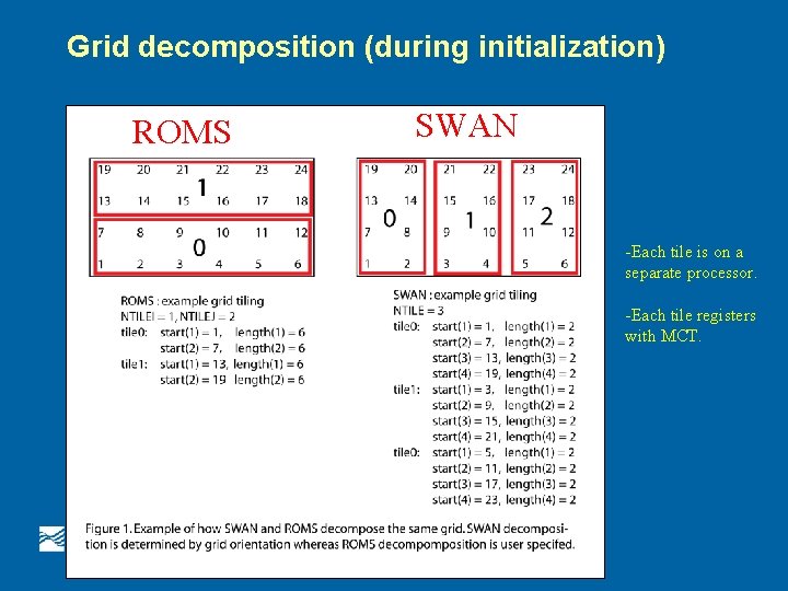
Grid decomposition (during initialization) ROMS SWAN -Each tile is on a separate processor. -Each tile registers with MCT.

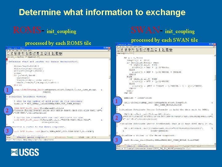
Determine what information to exchange ROMS- init_coupling SWAN- init_coupling processed by each SWAN tile processed by each ROMS tile 1 1 2 2 3 3

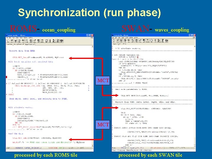
Synchronization (run phase) ROMS- ocean_coupling SWAN- waves_coupling MCT processed by each ROMS tile processed by each SWAN tile

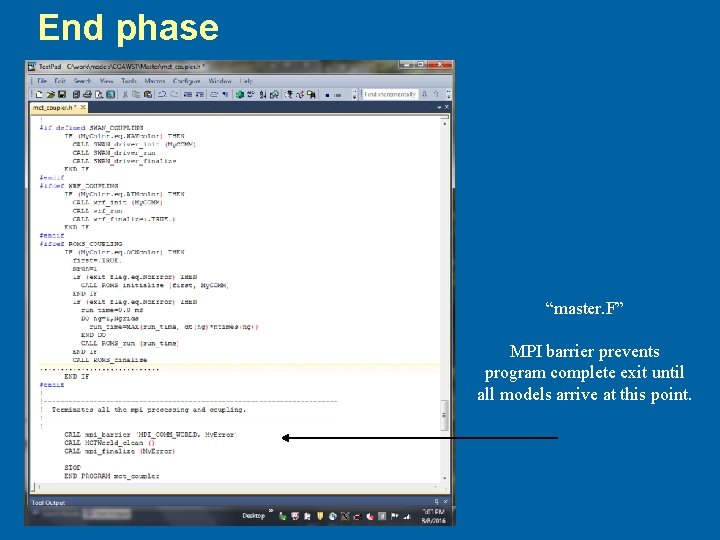
End phase “master. F” MPI barrier prevents program complete exit until all models arrive at this point.

SCRIP grid interpolation http: //oceans 11. lanl. gov/trac/SCRIP • Needed when you run more than 1 model and the models are on different grids. • We started with SCRIP from LANL. • We adapted the code to read model grids, and write out one Net. CDF file with all the interpolation weights. • We use the ‘group’ capability in Net. CDF 4.

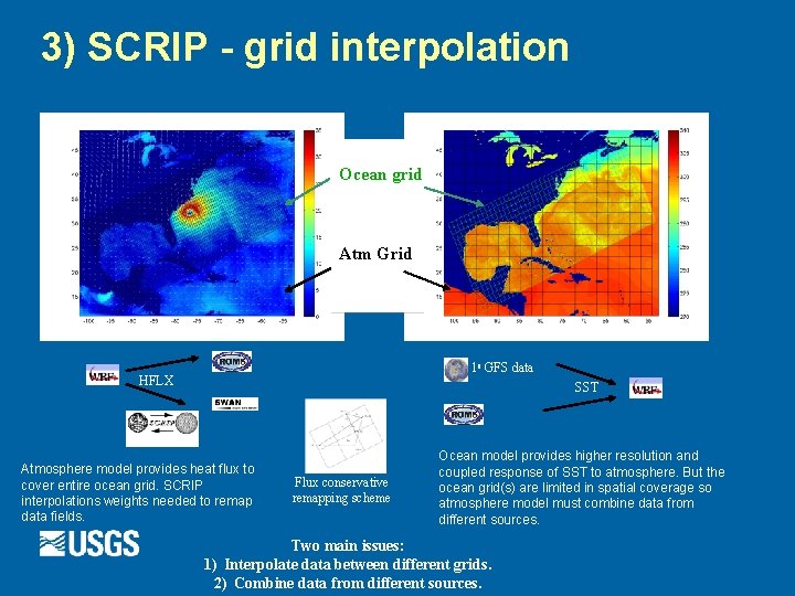
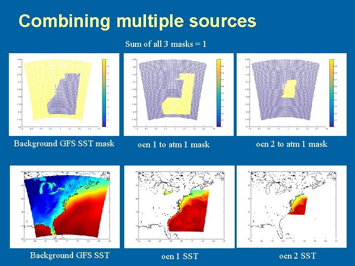
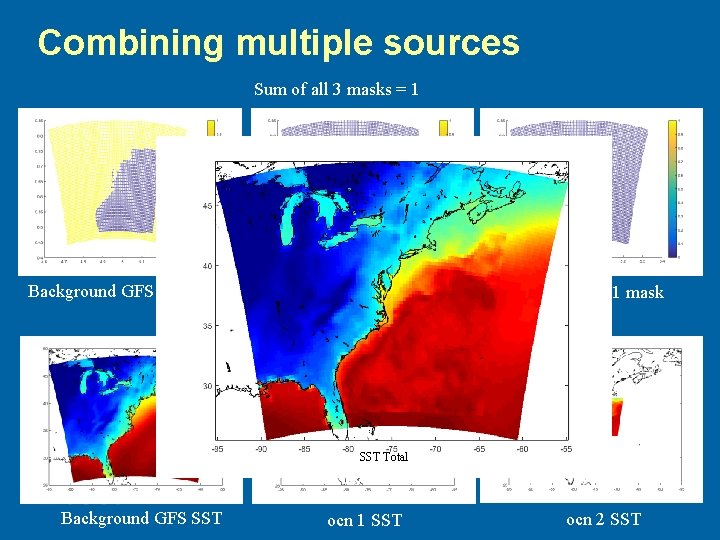
3) SCRIP - grid interpolation Ocean grid Atm Grid 10 GFS data HFLX SST Atmosphere model provides heat flux to cover entire ocean grid. SCRIP interpolations weights needed to remap data fields. Flux conservative remapping scheme Ocean model provides higher resolution and coupled response of SST to atmosphere. But the ocean grid(s) are limited in spatial coverage so atmosphere model must combine data from different sources. Two main issues: 1) Interpolate data between different grids. 2) Combine data from different sources.

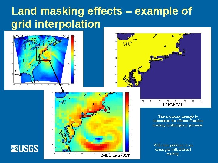
Land masking effects – example of grid interpolation LANDMASK This is a coarse example to demonstrate the effects of land/sea masking on atmospheric processes. Bottom stress (UST) Will cause problems on an ocean grid with different masking.

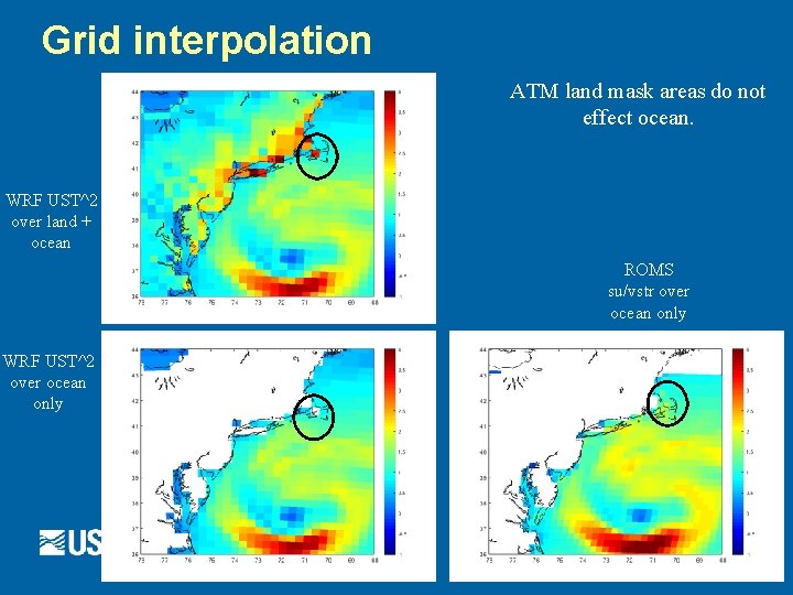
Grid interpolation ATM land mask areas do not effect ocean. WRF UST^2 over land + ocean ROMS su/vstr over ocean only WRF UST^2 over ocean only

Combining multiple sources Sum of all 3 masks = 1 Background GFS SST mask Background GFS SST ocn 1 to atm 1 mask ocn 1 SST ocn 2 to atm 1 mask ocn 2 SST

Combining multiple sources Sum of all 3 masks = 1 Background GFS SST mask ocn 1 to atm 1 mask ocn 2 to atm 1 mask SST Total Background GFS SST ocn 1 SST ocn 2 SST

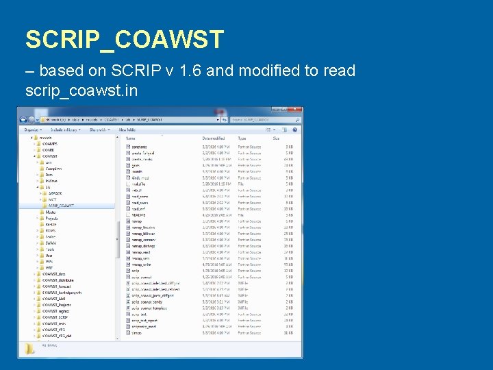
SCRIP_COAWST – based on SCRIP v 1. 6 and modified to read scrip_coawst. in

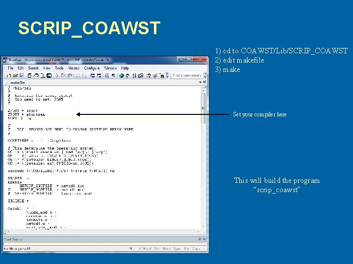
SCRIP_COAWST 1) cd to COAWST/Lib/SCRIP_COAWST 2) edit makefile 3) make Set your compiler here This will build the program “scrip_coawst”

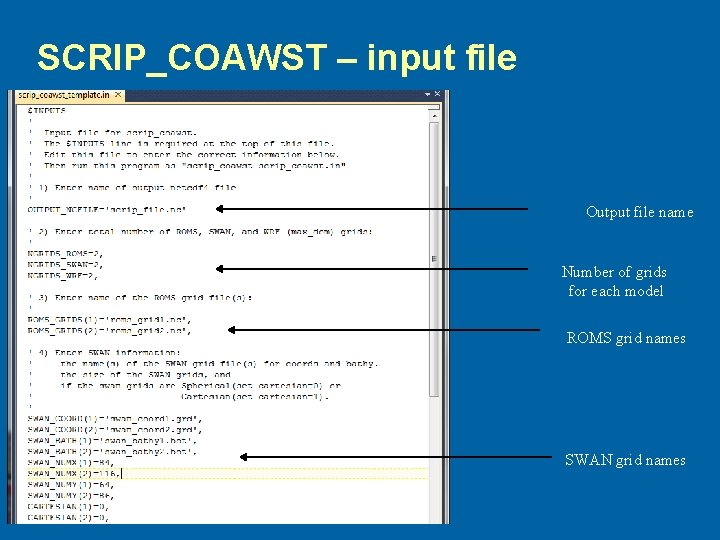
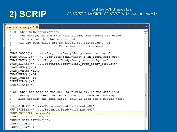
SCRIP_COAWST – input file Output file name Number of grids for each model ROMS grid names SWAN grid names

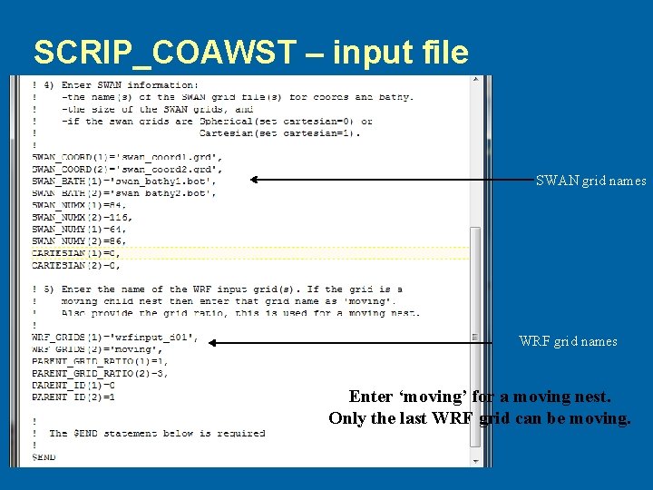
SCRIP_COAWST – input file SWAN grid names WRF grid names Enter ‘moving’ for a moving nest. Only the last WRF grid can be moving.

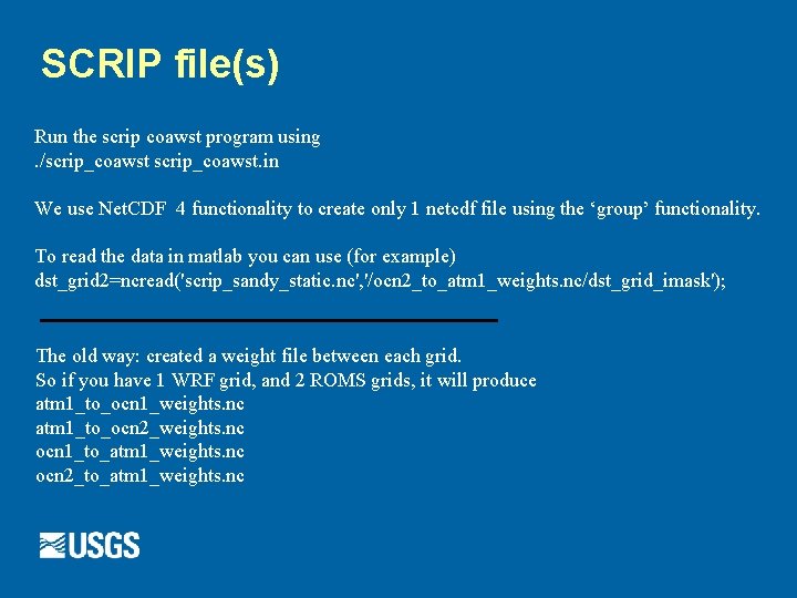
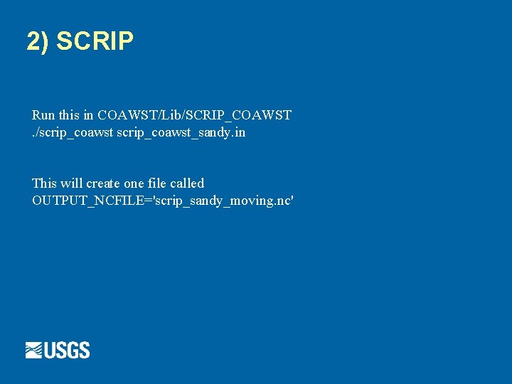
SCRIP file(s) Run the scrip coawst program using. /scrip_coawst. in We use Net. CDF 4 functionality to create only 1 netcdf file using the ‘group’ functionality. To read the data in matlab you can use (for example) dst_grid 2=ncread('scrip_sandy_static. nc', '/ocn 2_to_atm 1_weights. nc/dst_grid_imask'); The old way: created a weight file between each grid. So if you have 1 WRF grid, and 2 ROMS grids, it will produce atm 1_to_ocn 1_weights. nc atm 1_to_ocn 2_weights. nc ocn 1_to_atm 1_weights. nc ocn 2_to_atm 1_weights. nc

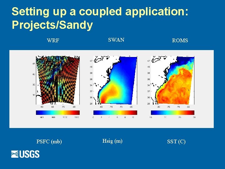
Setting up a coupled application: Projects/Sandy WRF PSFC (mb) SWAN Hsig (m) ROMS SST (C)

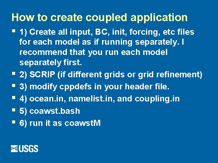
How to create coupled application § 1) Create all input, BC, init, forcing, etc files § § § for each model as if running separately. I recommend that you run each model separately first. 2) SCRIP (if different grids or grid refinement) 3) modify cppdefs in your header file. 4) ocean. in, namelist. in, and coupling. in 5) coawst. bash 6) run it as coawst. M

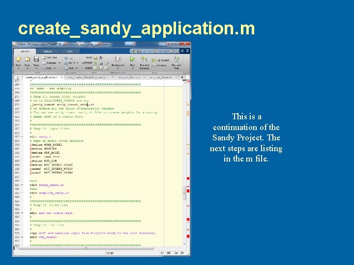
create_sandy_application. m This is a continuation of the Sandy Project. The next steps are listing in the m file.

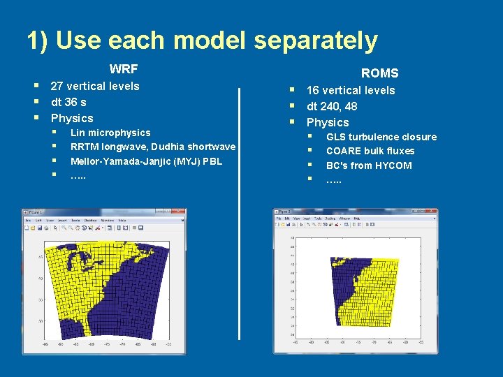
1) Use each model separately WRF § § § 27 vertical levels dt 36 s Physics § § Lin microphysics RRTM longwave, Dudhia shortwave Mellor-Yamada-Janjic (MYJ) PBL …. . ROMS § § § 16 vertical levels dt 240, 48 Physics § § GLS turbulence closure COARE bulk fluxes BC's from HYCOM …. .

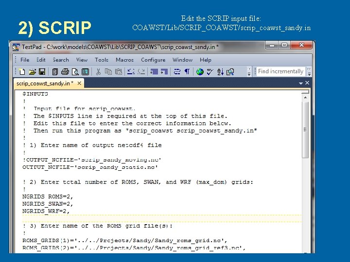
2) SCRIP Edit the SCRIP input file: COAWST/Lib/SCRIP_COAWST/scrip_coawst_sandy. in

2) SCRIP Edit the SCRIP input file: COAWST/Lib/SCRIP_COAWST/scrip_coawst_sandy. in

2) SCRIP Run this in COAWST/Lib/SCRIP_COAWST. /scrip_coawst_sandy. in This will create one file called OUTPUT_NCFILE='scrip_sandy_moving. nc'

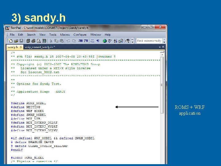
3) sandy. h ROMS + WRF application

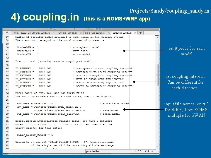
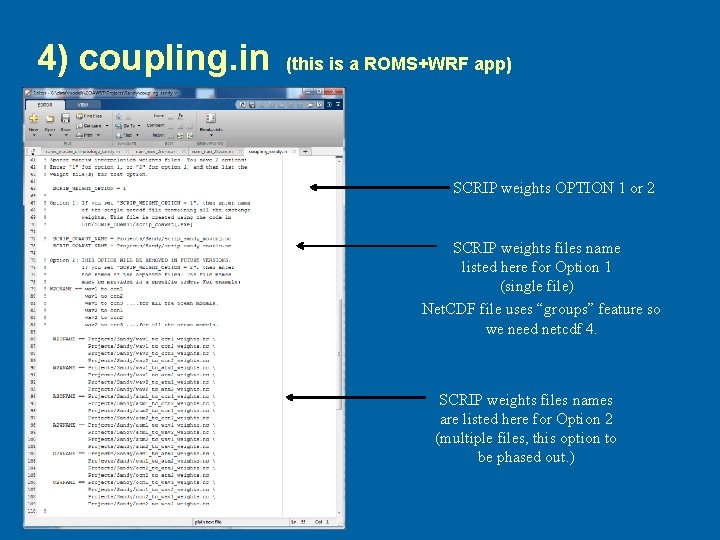
4) coupling. in Projects/Sandy/coupling_sandy. in (this is a ROMS+WRF app) set # procs for each model set coupling interval. Can be different for each direction. input file names. only 1 for WRF, 1 for ROMS, multiple for SWAN

4) coupling. in (this is a ROMS+WRF app) SCRIP weights OPTION 1 or 2 SCRIP weights files name listed here for Option 1 (single file) Net. CDF file uses “groups” feature so we need netcdf 4. SCRIP weights files names are listed here for Option 2 (multiple files, this option to be phased out. )

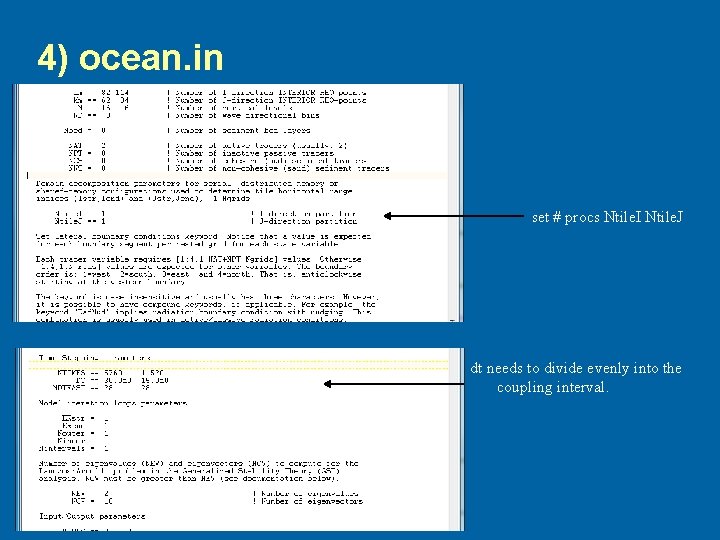
4) ocean. in set # procs Ntile. I Ntile. J Model dt needs to divide evenly into the coupling interval.

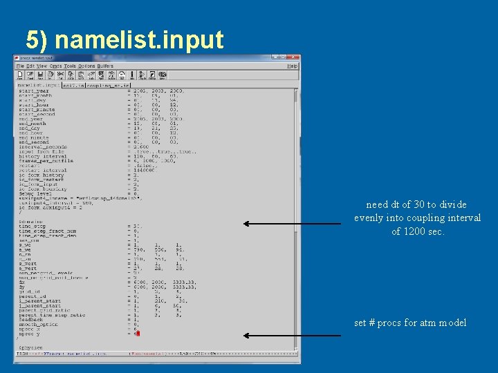
5) namelist. input need dt of 30 to divide evenly into coupling interval of 1200 sec. set # procs for atm model

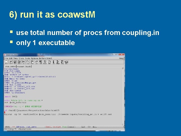
6) run it as coawst. M § § use total number of procs from coupling. in only 1 executable

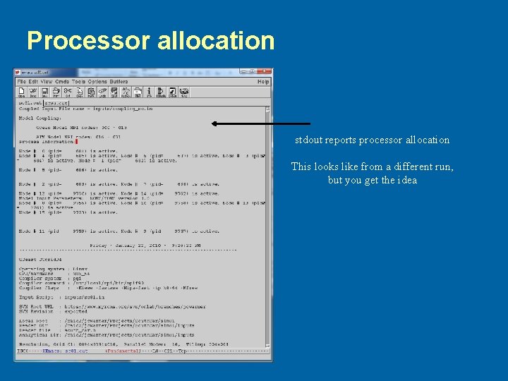
Processor allocation stdout reports processor allocation This looks like from a different run, but you get the idea

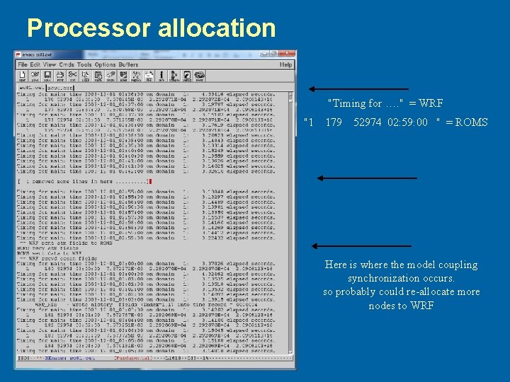
Processor allocation "Timing for …. " = WRF "1 179 52974 02: 59: 00 " = ROMS Here is where the model coupling synchronization occurs. so probably could re-allocate more nodes to WRF

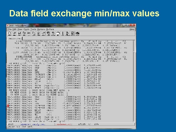
Data field exchange min/max values

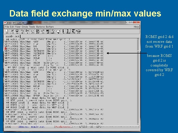
Data field exchange min/max values ROMS grid 2 did not receive data from WRF grid 1 because ROMS grid 2 is completely covered by WRF grid 2