Counter propagation network CPN 5 3 Basic idea
 (§ 5. 3) • Basic idea of CPN – Purpose:")
Counter propagation network (CPN) (§ 5. 3) • Basic idea of CPN – Purpose: fast and coarse approximation of vector mapping • not to map any given x to its with given precision, • input vectors x are divided into clusters/classes. • each cluster of x has one output y, which is (hopefully) the average of for all x in that class. – Architecture: Simple case: FORWARD ONLY CPN, x 1 xi z 1 w k, i xn from input to hidden (class) zk zp y 1 v j, k yj ym from hidden (class) to output
 where is the")
– Learning in two phases: – training sample (x, d ) where is the desired precise mapping – Phase 1: weights coming into hidden nodes are trained by competitive learning to become the representative vector of a cluster of input vectors x: (use only x, the input part of (x, d )) 1. For a chosen x, feedforward to determined the winning 2. 3. Reduce , then repeat steps 1 and 2 until stop condition is met – Phase 2: weights going out of hidden nodes are trained by delta rule to be an average output of where x is an input vector that causes to win (use both x and d). 1. For a chosen x, feedforward to determined the winning 2. (optional) 3. 4. Repeat steps 1 – 3 until stop condition is met
 and supervised")
Notes • A combination of both unsupervised learning (for in phase 1) and supervised learning (for in phase 2). • After phase 1, clusters are formed among sample input x , each is a representative of a cluster (average). • After phase 2, each cluster k maps to an output vector y, which is the average of • View phase 2 learning as following delta rule •


• After training, the networks like a look-up of math table. – For any input x, find a region where x falls (represented by the wining z node); – use the region as the index to look-up the table for the function value. – CPN works in multi-dimensional input space – More cluster nodes (z), more accurate mapping. – Training is much faster than BP – May have linear separability problem

Full CPN • If both we can establish bi-directional approximation • Two pairs of weights matrices: W(x to z) and V(z to y) for approx. map x to U(y to z) and T(z to x) for approx. map y to • When training sample (x, y) is applied ( ), they can jointly determine the winner zk* or separately for
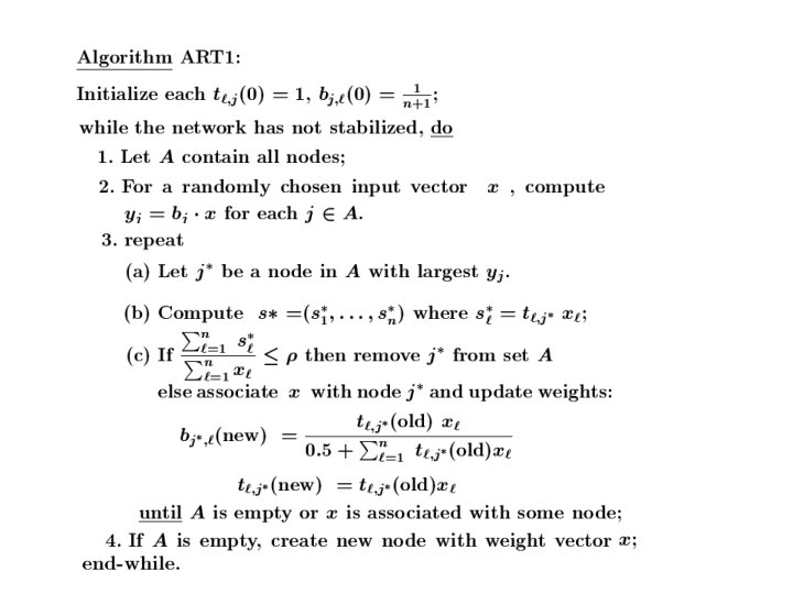
 (§ 5. 4) • ART 1: for binary patterns; ART")
Adaptive Resonance Theory (ART) (§ 5. 4) • ART 1: for binary patterns; ART 2: for continuous patterns • Motivations: Previous methods have the following problems: 1. Number of class nodes is pre-determined and fixed. – Under- and over- classification may result from training – Some nodes may have empty classes. – no control of the degree of similarity of inputs grouped in one class. 2. Training is non-incremental: – with a fixed set of samples, – adding new samples often requires re-train the network with the enlarged training set until a new stable state is reached.

• Ideas of ART model: – suppose the input samples have been appropriately classified into k clusters (say by some fashion of competitive learning). – each weight vector is a representative (average) of all samples in that cluster. – when a new input vector x arrives 1. Find the winner j* among all k cluster nodes 2. Compare with x if they are sufficiently similar (x resonates with class j*), then update based on else, find/create a free class node and make x as its first member.

• To achieve these, we need: – a mechanism for testing and determining (dis)similarity between x and. – a control for finding/creating new class nodes. – need to have all operations implemented by units of local computation. • Only the basic ideas are presented – Simplified from the original ART model – Some of the control mechanisms realized by various specialized neurons are done by logic statements of the algorithm

ART 1 Architecture

Working of ART 1 • 3 phases after each input vector x is applied • Recognition phase: determine the winner cluster for x – Using bottom-up weights b – Winner j* with max yj* = bj* x – x is tentatively classified to cluster j* – the winner may be far away from x (e. g. , |tj* - x| is unacceptably large)
 • Comparison phase: – Compute similarity using top-down")
Working of ART 1 (3 phases) • Comparison phase: – Compute similarity using top-down weights t: vector: – If (# of 1’s in s)|/(# of 1’s in x) > ρ, accept the classification, update bj* and tj* – else: remove j* from further consideration, look for other potential winner or create a new node with x as its first patter.
 bottom up: top down:")
• Weight update/adaptive phase – Initial weight: (no bias) bottom up: top down: – When a resonance occurs with – If k sample patterns are clustered to node j then = pattern whose 1’s are common to all these k samples
 Node 1 wins")
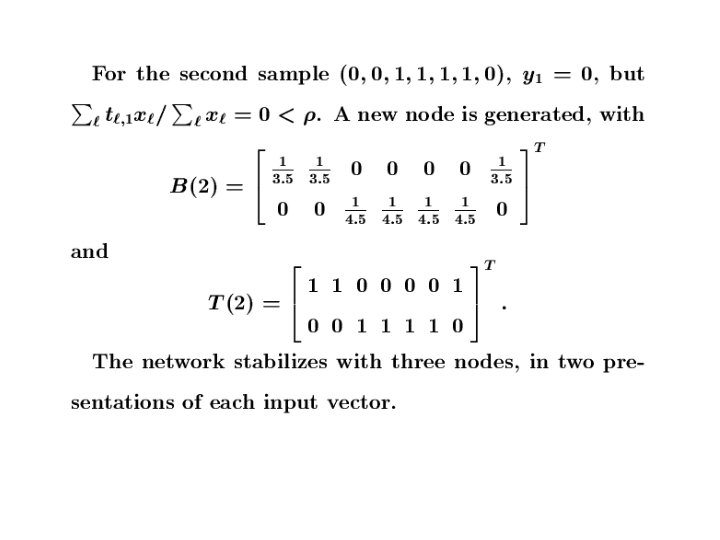
• Example for input x(1) Node 1 wins

Notes 1. Classification as a search process 2. No two classes have the same b and t 3. Outliers that do not belong to any cluster will be assigned separate nodes 4. Different ordering of sample input presentations may result in different classification. 5. Increase of r increases # of classes learned, and decreases the average class size. 6. Classification may shift during search, will reach stability eventually. 7. There are different versions of ART 1 with minor variations 8. ART 2 is the same in spirit but different in details.

ART 1 Architecture + + - R + + + G 1 G 2 +

• cluster units: competitive, receive input vector x through weights b: to determine winner j. • input units: placeholder or external inputs • interface units: – pass s to x as input vector for classification by – compare x and – controlled by gain control unit G 1 • • Needs to sequence three phases (by control units G 1, G 2, and R)

R = 0: resonance occurs, update and R = 1: fails similarity test, inhibits J from further computation
- Slides: 20