COT 5611 Operating Systems Design Principles Spring 2014

COT 5611 Operating Systems Design Principles Spring 2014 Dan C. Marinescu Office: HEC 304 Office hours: M-Wd 3: 30 – 5: 30 PM

Lecture 14 n Reading assignment: ¨ n Chapter 8 from the on-line text Last time: Control mechanisms and decisions in the Internet. ¨ The network layer ¨ The end-to-end layer ¨ 10/24/2021 Lecture 14 2

Today n Reliability and fault tolerance 10/24/2021 Lecture 14 3

Reliable Systems from Unreliable Components n n Problem investigated first in mid 1940 s by John von Neumann. Steps to build reliable systems ¨ Error detection n Network protocols (link and end-to-end) ¨ Error containment – limit the effect of errors n Enforced modularity: client-server architectures, virtual memory, etc. ¨ Error masking – ensure correct operation in the presence of errors n Network protocols: error correction, repetition, interpolation for data cu real-time constrains 10/24/2021 Lecture 14 4

Faults and errors n Fault a flaw with the potential to cause problems; occurs when an error is not detected and masked ¨ ¨ ¨ n Software Hardware Design e. g. , under-provisioning resources Implementation e. g. , setting the wrong device priorities on a bus Operation setting the wrong date Environment failure of the cooling system may cause intermittent memory errors Types of faults Latent not active now ¨ Active ¨ n n n Error the consequence of an active fault. Failure inability to produce the desired result. Distinction between failure and fault related to modularity a fault of a component may lead to the failure of the entire system but it may be detected and masked by other components. 10/24/2021 Lecture 14 5

Error containment in a layered system n Several design strategies are possible. The layer where an error occurs: Masks the error correct it internally so that the higher layer is not aware of it. ¨ Detects the error and report its to the higher layer fail-fast. ¨ Stops fail-stop. ¨ Does nothing. ¨ n Types of faults Transient (caused by passing external condition)/Persistent ¨ Soft /Hard Can be masked or not by a retry. ¨ Intermittent occurs only occasionally and it is not reproducible ¨ n Latency of a fault – time until a fault causes an error ¨ A long latency may allow errors to accumulate and defeat periodic error correction 10/24/2021 Lecture 14 6

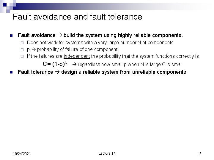
Fault avoidance and fault tolerance n Fault avoidance build the system using highly reliable components. Does not work for systems with a very large number N of components ¨ p probability of failure of one component ¨ If the failures are independent the probability that the system functions correctly is ¨ C= (1 -p)N n regardless how small p when N is large C is small Fault tolerance design a reliable system from unreliable components 10/24/2021 Lecture 14 7

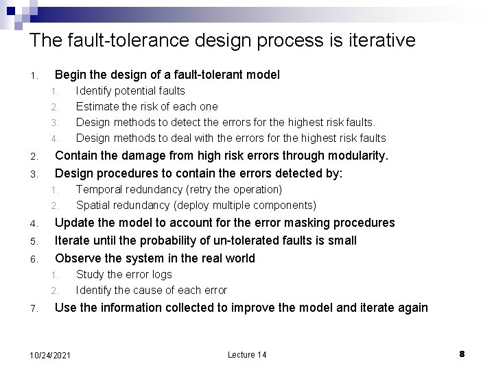
The fault-tolerance design process is iterative 1. Begin the design of a fault-tolerant model 1. 2. 3. 4. 2. 3. Contain the damage from high risk errors through modularity. Design procedures to contain the errors detected by: 1. 2. 4. 5. 6. Temporal redundancy (retry the operation) Spatial redundancy (deploy multiple components) Update the model to account for the error masking procedures Iterate until the probability of un-tolerated faults is small Observe the system in the real world 1. 2. 7. Identify potential faults Estimate the risk of each one Design methods to detect the errors for the highest risk faults. Design methods to deal with the errors for the highest risk faults Study the error logs Identify the cause of each error Use the information collected to improve the model and iterate again 10/24/2021 Lecture 14 8

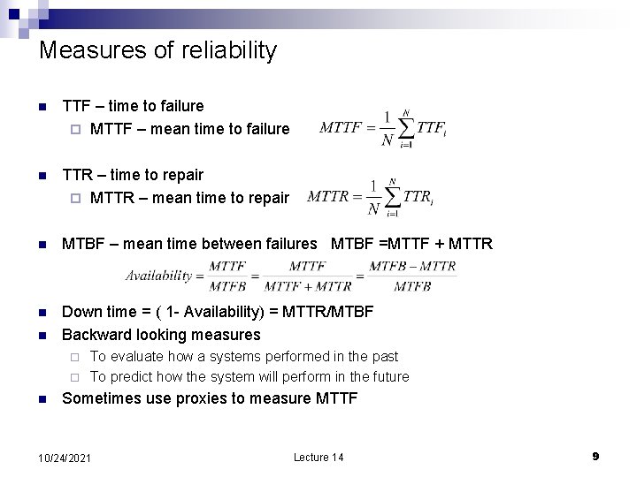
Measures of reliability n TTF – time to failure ¨ MTTF – mean time to failure n TTR – time to repair ¨ MTTR – mean time to repair n MTBF – mean time between failures MTBF =MTTF + MTTR n Down time = ( 1 - Availability) = MTTR/MTBF Backward looking measures n To evaluate how a systems performed in the past ¨ To predict how the system will perform in the future ¨ n Sometimes use proxies to measure MTTF 10/24/2021 Lecture 14 9

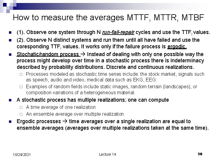
How to measure the averages MTTF, MTTR, MTBF n n n (1). Observe one system through N run-fail-repair cycles and use the TTFi values. (2). Observe N distinct systems and run them until all have failed and use the coresponding TTFi values. It works only if the failure process is ergodic. Stochatic/random process Instead of dealing with only one possible way the process might develop over time in a stochastic process there is indeterminacy described by probability distributions. Discrete and continuous realizations. Processes modeled as stochastic time series include: the stock market, signals such as speech, audio and video, medical data such as EKG, EEG. ¨ Examples of random fields include static images, random terrain (landscapes), or composition variations of a heterogeneous material. ¨ n A stochastic process has multiple realizations; one can compute A time average of one realization ¨ An ensemble average over multiple realization ¨ n Ergodic processes time averages over a single realization are equal to ensemble averages (averages over multiple realizations taken at the same time). 10/24/2021 Lecture 14 10

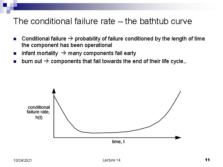
The conditional failure rate – the bathtub curve n n n Conditional failure probability of failure conditioned by the length of time the component has been operational infant mortality many components fail early burn out components that fail towards the end of their life cycle, . 10/24/2021 Lecture 14 11

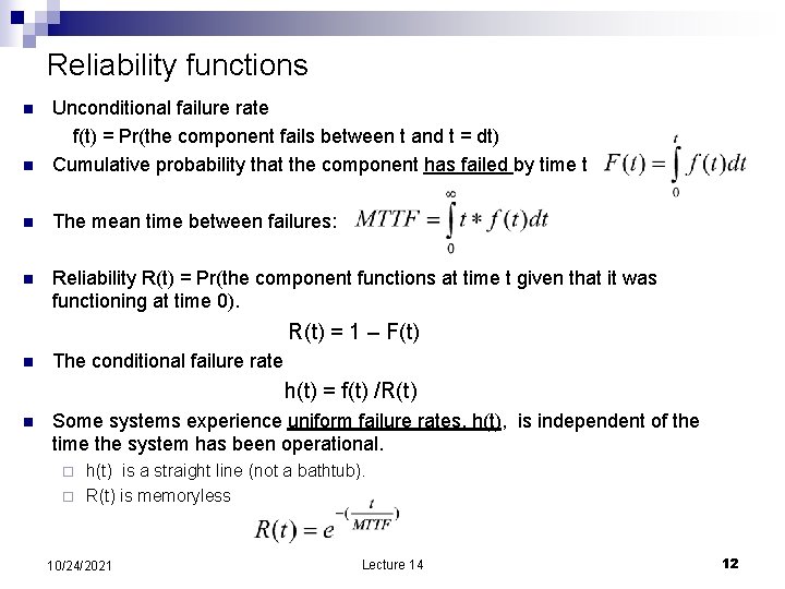
Reliability functions n Unconditional failure rate f(t) = Pr(the component fails between t and t = dt) Cumulative probability that the component has failed by time t n The mean time between failures: n Reliability R(t) = Pr(the component functions at time t given that it was functioning at time 0). n R(t) = 1 – F(t) n The conditional failure rate h(t) = f(t) /R(t) n Some systems experience uniform failure rates, h(t), is independent of the time the system has been operational. h(t) is a straight line (not a bathtub). ¨ R(t) is memoryless ¨ 10/24/2021 Lecture 14 12

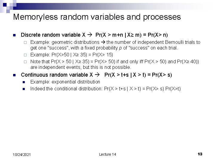
Memoryless random variables and processes n Discrete random variable X Pr(X > m+n | X≥ m) = Pr(X> n) Example: geometric distributions the number of independent Bernoulli trials to get one "success", with a fixed probability p of "success" on each trial. ¨ Example: Pr(X>50 | X≥ 35) = Pr(X> 15) ¨ Note that Pr(X > 50 | X≥ 35) = Pr(X> 50) if and only iff Pr(X > 50) and Pr(X≥ 40)) are independent events, but this is not possible. ¨ n Continuous random variable X Pr(X > t+s | X > t) = Pr(X> s) n n Example: exponential distribution Indeed the conditional distribution: Pr(X > t+s | X > t) = Pr(X> s) Pr(X>t) 10/24/2021 Lecture 14 13

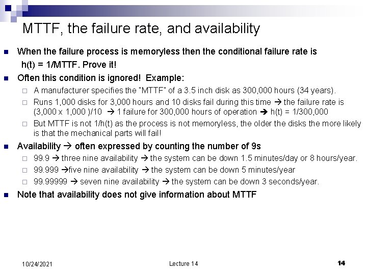
MTTF, the failure rate, and availability n n When the failure process is memoryless then the conditional failure rate is h(t) = 1/MTTF. Prove it! Often this condition is ignored! Example: A manufacturer specifies the “MTTF” of a 3. 5 inch disk as 300, 000 hours (34 years). ¨ Runs 1, 000 disks for 3, 000 hours and 10 disks fail during this time the failure rate is (3, 000 x 1, 000 )/10 1 failure for 300, 000 hours of operation h(t) = 1/300, 000 ¨ But MTTF is not 1/h(t) as the process is not memoryless, the older the disks the more likely is that the mechanical parts will fail! ¨ n Availability often expressed by counting the number of 9 s 99. 9 three nine availability the system can be down 1. 5 minutes/day or 8 hours/year. ¨ 99. 999 five nine availability the system can be down 5 minutes/year ¨ 99. 99999 seven nine availability the system can be down 3 seconds/year. ¨ n Note that availability does not give information about MTTF 10/24/2021 Lecture 14 14

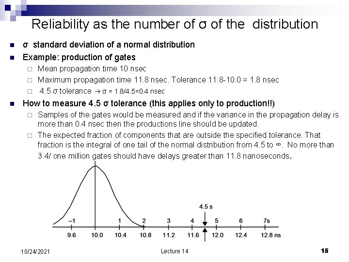
Reliability as the number of σ of the distribution n n σ standard deviation of a normal distribution Example: production of gates Mean propagation time 10 nsec ¨ Maximum propagation time 11. 8 nsec. Tolerance 11. 8 -10. 0 = 1. 8 nsec ¨ 4. 5 σ tolerance σ = 1. 8/4. 5=0. 4 nsec ¨ n How to measure 4. 5 σ tolerance (this applies only to production!!) Samples of the gates would be measured and if the variance in the propagation delay is more than 0. 4 nsec then the productions line should be updated. ¨ The expected fraction of components that are outside the specified tolerance. That fraction is the integral of one tail of the normal distribution from 4. 5 to ∞. No more than 3. 4/ one million gates should have delays greater than 11. 8 nanoseconds. ¨ 10/24/2021 Lecture 14 15

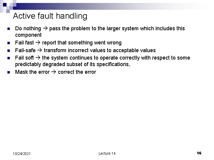
Active fault handling n n n Do nothing pass the problem to the larger system which includes this component Fail fast report that something went wrong Fail-safe transform incorrect values to acceptable values Fail soft the system continues to operate correctly with respect to some predictably degraded subset of its specifications, Mask the error correct the error 10/24/2021 Lecture 14 16

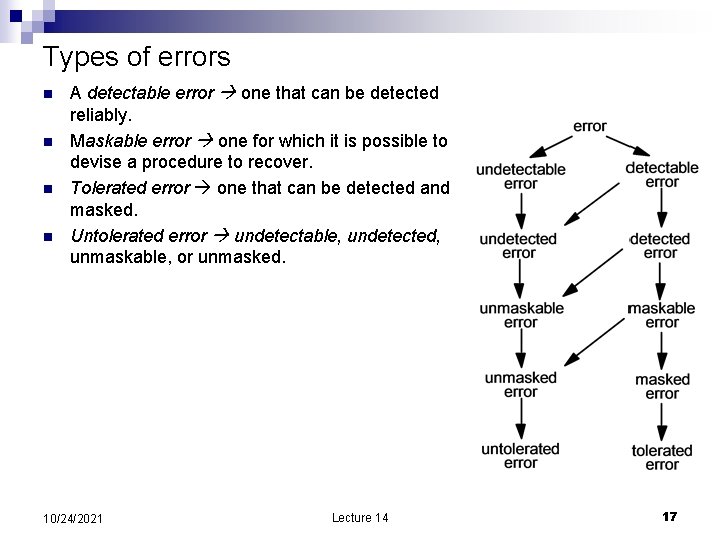
Types of errors n n A detectable error one that can be detected reliably. Maskable error one for which it is possible to devise a procedure to recover. Tolerated error one that can be detected and masked. Untolerated error undetectable, undetected, unmaskable, or unmasked. 10/24/2021 Lecture 14 17

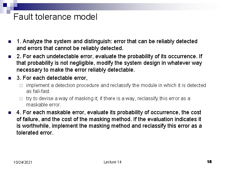
Fault tolerance model n n n 1. Analyze the system and distinguish: error that can be reliably detected and errors that cannot be reliably detected. 2. For each undetectable error, evaluate the probability of its occurrence. If that probability is not negligible, modify the system design in whatever way necessary to make the error reliably detectable. 3. For each detectable error, implement a detection procedure and reclassify the module in which it is detected as fail-fast. ¨ try to devise a way of masking it; if there is a way, reclassify this error as a maskable error. ¨ n 4. For each maskable error, evaluate its probability of occurrence, the cost of failure, and the cost of the masking method. If the evaluation indicates it is worthwhile, implement the masking method and reclassify this error as a tolerated error. 10/24/2021 Lecture 14 18

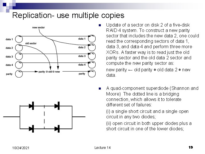
Replication- use multiple copies 10/24/2021 n Update of a sector on disk 2 of a five-disk RAID 4 system. To construct a new parity sector that includes the new data 2, one could read the corresponding sectors of data 1, data 3, and data 4 and perform three more XORs. A faster way is to read just the old parity sector and the old data 2 sector and compute the new parity sector as: new parity ← old parity ⊕ old data 2 ⊕ new data. n A quad-component superdiode (Shannon and Moore) The dotted line is a bridging connection, which allows it to tolerate different set of failures: (i) a single short circuit and a single open circuit in any two diodes; (ii) open circuit in both upper diodes plus a short circuit in one of the lower diodes; Lecture 14 19

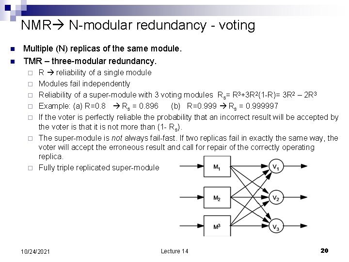
NMR N-modular redundancy - voting n n Multiple (N) replicas of the same module. TMR – three-modular redundancy. ¨ ¨ ¨ ¨ R reliability of a single module Modules fail independently Reliability of a super-module with 3 voting modules Rs= R 3+3 R 2(1 -R)= 3 R 2 – 2 R 3 Example: (a) R=0. 8 Rs = 0. 896 (b) R=0. 999 Rs = 0. 999997 If the voter is perfectly reliable the probability that an incorrect result will be accepted by the voter is that it is not more than (1 - Rs). The super-module is not always fail-fast. If two replicas fail in exactly the same way, the voter will accept the erroneous result and call for repair of the correctly operating replica. Fully triple replicated super-module 10/24/2021 Lecture 14 20